

26 Eigen Stresses and Dislocations
289
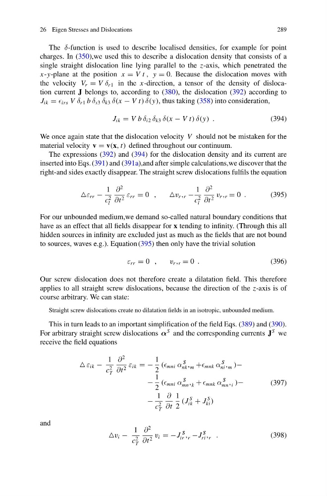
The δ-function is used to describe localised densities, for example for point
charges. In (350),we used this to describe a dislocation density that consists of a
single straight dislocation line lying parallel to the z-axis, which penetrated the
x-y-plane at the position x = V t , y = 0. Because the dislocation moves with
the velocity V r = V δ r 1 in the x-direction, a tensor of the density of dislocation current J belongs to, according to (380), the dislocation (392) according to
J ik = irs V δ r 1 b δ s3 δ k3 δ(x − V t) δ(y), thus taking (358) into consideration,
J ik = V b δ i2 δ k3 δ(x − V t) δ(y) .
(394)
We once again state that the dislocation velocity V should not be mistaken for the
material velocity v = v(x, t) defined throughout our continuum.
The expressions (392) and (394) for the dislocation density and its current are
inserted into Eqs. (391) and (391a),and after simple calculations,we discover that the
right-and sides exactly disappear. The straight screw dislocations fulfils the equation
ε rr −
1
c
2
l
∂
2
∂t 2 ε rr = 0 ,
v r , r −
1
c
2
l
∂
2
∂t 2 v r , r = 0 .
(395)
For our unbounded medium,we demand so-called natural boundary conditions that
have as an effect that all fields disappear for x tending to infinity. (Through this all
hidden sources in infinity are excluded just as much as the fields that are not bound
to sources, waves e.g.). Equation (395) then only have the trivial solution
ε rr = 0 ,
v r , r = 0 .
(396)
Our screw dislocation does not therefore create a dilatation field. This therefore
applies to all straight screw dislocations, because the direction of the z-axis is of
course arbitrary. We can state:
Straight screw dislocations create no dilatation fields in an isotropic, unbounded medium.
This in turn leads to an important simplification of the field Eqs. (389) and (390).
For arbitrary straight screw dislocations α
S and the corresponding currents J
S we
receive the field equations
ε ik −
1
c
2
T
∂
2
∂t 2 ε ik = −
1
2
( mni α
S
nk ,
S
m + mnk α
S
ni ,
S
m )−
−
1
2
( mni α
S
mn ,
S
k + mnk α
S
mn ,
S
i )−
−
1
c
2
T
∂
∂t
1
2
(J
S
ik + J
S
ki )
(397)
and
v i −
1
c
2
T
∂
2
∂t 2 v i = −J
S
ir ,
S
r −J
S
ri ,
S
r .
(398)
289
The δ-function is used to describe localised densities, for example for point
charges. In (350),we used this to describe a dislocation density that consists of a
single straight dislocation line lying parallel to the z-axis, which penetrated the
x-y-plane at the position x = V t , y = 0. Because the dislocation moves with
the velocity V r = V δ r 1 in the x-direction, a tensor of the density of dislocation current J belongs to, according to (380), the dislocation (392) according to
J ik = irs V δ r 1 b δ s3 δ k3 δ(x − V t) δ(y), thus taking (358) into consideration,
J ik = V b δ i2 δ k3 δ(x − V t) δ(y) .
(394)
We once again state that the dislocation velocity V should not be mistaken for the
material velocity v = v(x, t) defined throughout our continuum.
The expressions (392) and (394) for the dislocation density and its current are
inserted into Eqs. (391) and (391a),and after simple calculations,we discover that the
right-and sides exactly disappear. The straight screw dislocations fulfils the equation
ε rr −
1
c
2
l
∂
2
∂t 2 ε rr = 0 ,
v r , r −
1
c
2
l
∂
2
∂t 2 v r , r = 0 .
(395)
For our unbounded medium,we demand so-called natural boundary conditions that
have as an effect that all fields disappear for x tending to infinity. (Through this all
hidden sources in infinity are excluded just as much as the fields that are not bound
to sources, waves e.g.). Equation (395) then only have the trivial solution
ε rr = 0 ,
v r , r = 0 .
(396)
Our screw dislocation does not therefore create a dilatation field. This therefore
applies to all straight screw dislocations, because the direction of the z-axis is of
course arbitrary. We can state:
Straight screw dislocations create no dilatation fields in an isotropic, unbounded medium.
This in turn leads to an important simplification of the field Eqs. (389) and (390).
For arbitrary straight screw dislocations α
S and the corresponding currents J
S we
receive the field equations
ε ik −
1
c
2
T
∂
2
∂t 2 ε ik = −
1
2
( mni α
S
nk ,
S
m + mnk α
S
ni ,
S
m )−
−
1
2
( mni α
S
mn ,
S
k + mnk α
S
mn ,
S
i )−
−
1
c
2
T
∂
∂t
1
2
(J
S
ik + J
S
ki )
(397)
and
v i −
1
c
2
T
∂
2
∂t 2 v i = −J
S
ir ,
S
r −J
S
ri ,
S
r .
(398)