

272
25 Elastic Displacements and Waves
ρ
∂
2 s i
∂t 2 = C ikrs s r , sk + f i .
(342b)
If we have a case where a displacement vector s does not exist, we must go back to
Eq. (341) and receive,
ρ
∂
∂t
v i = C ikrs s r , sk + f i .
(343)
We formulate the following equation by differentiating the above Eq. (343) for later
application,
ρ
∂ 2
∂t 2
1
2
(v i , j +v j , i )
=
1
2
C ikrs ε rs , k j +C jkrs ε rs , ki
+
1
2
f i , j + f j , i
. (343a)
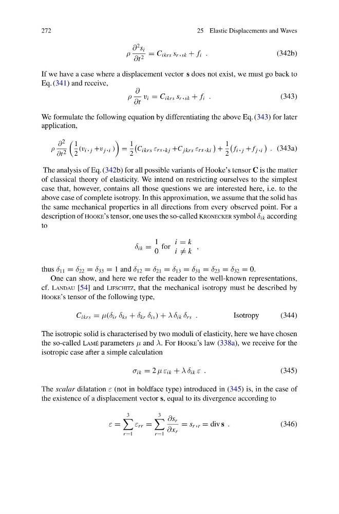
The analysis of Eq. (342b) for all possible variants of Hooke’s tensor C is the matter
of classical theory of elasticity. We intend on restricting ourselves to the simplest
case that, however, contains all those questions we are interested here, i.e. to the
above case of complete isotropy. In this approximation, we assume that the solid has
the same mechanical properties in all directions from every observed point. For a
description of Hooke’s tensor, one uses the so-called Kronecker symbol δ ik according
to
δ ik =
1
0
for
i = k
i = k
,
thus δ 11 = δ 22 = δ 33 = 1 and δ 12 = δ 21 = δ 13 = δ 31 = δ 23 = δ 32 = 0.
One can show, and here we refer the reader to the well-known representations,
cf. Landau [54] and Lifschitz, that the mechanical isotropy must be described by
Hooke’s tensor of the following type,
C ikrs = μ(δ ir δ ks + δ kr δ is ) + λ δ ik δ rs .
Isotropy
(344)
The isotropic solid is characterised by two moduli of elasticity, here we have chosen
the so-called Lamé parameters μ and λ. For Hooke’s law (338a), we receive for the
isotropic case after a simple calculation
σ ik = 2 μ ε ik + λ δ ik ε .
(345)
The scalar dilatation ε (not in boldface type) introduced in (345) is, in the case of
the existence of a displacement vector s, equal to its divergence according to
ε =
3
r =1
ε rr =
3
r =1
∂s r
∂x r
= s r , r = div s .
(346)
25 Elastic Displacements and Waves
ρ
∂
2 s i
∂t 2 = C ikrs s r , sk + f i .
(342b)
If we have a case where a displacement vector s does not exist, we must go back to
Eq. (341) and receive,
ρ
∂
∂t
v i = C ikrs s r , sk + f i .
(343)
We formulate the following equation by differentiating the above Eq. (343) for later
application,
ρ
∂ 2
∂t 2
1
2
(v i , j +v j , i )
=
1
2
C ikrs ε rs , k j +C jkrs ε rs , ki
+
1
2
f i , j + f j , i
. (343a)
The analysis of Eq. (342b) for all possible variants of Hooke’s tensor C is the matter
of classical theory of elasticity. We intend on restricting ourselves to the simplest
case that, however, contains all those questions we are interested here, i.e. to the
above case of complete isotropy. In this approximation, we assume that the solid has
the same mechanical properties in all directions from every observed point. For a
description of Hooke’s tensor, one uses the so-called Kronecker symbol δ ik according
to
δ ik =
1
0
for
i = k
i = k
,
thus δ 11 = δ 22 = δ 33 = 1 and δ 12 = δ 21 = δ 13 = δ 31 = δ 23 = δ 32 = 0.
One can show, and here we refer the reader to the well-known representations,
cf. Landau [54] and Lifschitz, that the mechanical isotropy must be described by
Hooke’s tensor of the following type,
C ikrs = μ(δ ir δ ks + δ kr δ is ) + λ δ ik δ rs .
Isotropy
(344)
The isotropic solid is characterised by two moduli of elasticity, here we have chosen
the so-called Lamé parameters μ and λ. For Hooke’s law (338a), we receive for the
isotropic case after a simple calculation
σ ik = 2 μ ε ik + λ δ ik ε .
(345)
The scalar dilatation ε (not in boldface type) introduced in (345) is, in the case of
the existence of a displacement vector s, equal to its divergence according to
ε =
3
r =1
ε rr =
3
r =1
∂s r
∂x r
= s r , r = div s .
(346)