

40
Electrochemical Supercapacitors for Energy Storage and Delivery
+ Positive charge
– Negative charge
Solvent molecule
Electrode
Electrolyte solution
–
+
+
–
–
+ –
–
+
+
–
–
–
+
+
+
–
–
+
–
+
+
–
–
–
+ –
+
+
–
+
–
+
+
–
–
+
–
+
+ –
–
–
–
+
–
+
+
–
–
+
–
–
–
–
+
+
+
d OHP
+
+
+
d
d IHP
L diff
L diff
OHP
IHP
(a)
(b)
(c)
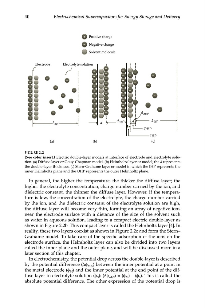
FIGURE 2.2
(See color insert.) Electric double-layer models at interface of electrode and electrolyte solution. (a) Diffuse layer or Gouy-Chapman model. (b) Helmholtz layer or model; the d represents
the double-layer thickness. (c) Stern-Grahame layer or model in which the IHP represents the
inner Helmholtz plane and the OHP represents the outer Helmholtz plane.
In general, the higher the temperature, the thicker the diffuse layer; the
higher the electrolyte concentration, charge number carried by the ion, and
dielectric constant, the thinner the diffuse layer. However, if the temperature is low, the concentration of the electrolyte, the charge number carried
by the ion, and the dielectric constant of the electrolyte solution are high,
the diffuse layer will become very thin, forming an array of negative ions
near the electrode surface with a distance of the size of the solvent such
as water in aqueous solution, leading to a compact electric double-layer as
shown in Figure 2.2b. This compact layer is called the Helmholtz layer [4]. In
reality, these two layers coexist as shown in Figure 2.2c and form the Stern–
Grahame model. To take care of the specific adsorption of the ions on the
electrode surface, the Helmholtz layer can also be divided into two layers
called the inner plane and the outer plane, and will be discussed more in a
later section of this chapter.
In electrochemistry, the potential drop across the double-layer is described
by the potential difference (Δϕ M/S ) between the inner potential at a point in
the metal electrode (ϕ M ) and the inner potential at the end point of the diffuse layer in electrolyte solution (ϕ S ): (Δϕ M/S ) = (ϕ M ) – (ϕ S ). This is called the
absolute potential difference. The other expression of the potential drop is
Electrochemical Supercapacitors for Energy Storage and Delivery
+ Positive charge
– Negative charge
Solvent molecule
Electrode
Electrolyte solution
–
+
+
–
–
+ –
–
+
+
–
–
–
+
+
+
–
–
+
–
+
+
–
–
–
+ –
+
+
–
+
–
+
+
–
–
+
–
+
+ –
–
–
–
+
–
+
+
–
–
+
–
–
–
–
+
+
+
d OHP
+
+
+
d
d IHP
L diff
L diff
OHP
IHP
(a)
(b)
(c)
FIGURE 2.2
(See color insert.) Electric double-layer models at interface of electrode and electrolyte solution. (a) Diffuse layer or Gouy-Chapman model. (b) Helmholtz layer or model; the d represents
the double-layer thickness. (c) Stern-Grahame layer or model in which the IHP represents the
inner Helmholtz plane and the OHP represents the outer Helmholtz plane.
In general, the higher the temperature, the thicker the diffuse layer; the
higher the electrolyte concentration, charge number carried by the ion, and
dielectric constant, the thinner the diffuse layer. However, if the temperature is low, the concentration of the electrolyte, the charge number carried
by the ion, and the dielectric constant of the electrolyte solution are high,
the diffuse layer will become very thin, forming an array of negative ions
near the electrode surface with a distance of the size of the solvent such
as water in aqueous solution, leading to a compact electric double-layer as
shown in Figure 2.2b. This compact layer is called the Helmholtz layer [4]. In
reality, these two layers coexist as shown in Figure 2.2c and form the Stern–
Grahame model. To take care of the specific adsorption of the ions on the
electrode surface, the Helmholtz layer can also be divided into two layers
called the inner plane and the outer plane, and will be discussed more in a
later section of this chapter.
In electrochemistry, the potential drop across the double-layer is described
by the potential difference (Δϕ M/S ) between the inner potential at a point in
the metal electrode (ϕ M ) and the inner potential at the end point of the diffuse layer in electrolyte solution (ϕ S ): (Δϕ M/S ) = (ϕ M ) – (ϕ S ). This is called the
absolute potential difference. The other expression of the potential drop is