

E,V
1.2
1.0
0.8
0.6
0.4
0.2
0.0
E i + v 2 λ 2
E i + v 1 λ 1
v 2 = 0.02 V.s
–1
v 1 = 0.005 V.s
–1
E i
λ 2
λ 1
0 20 40 60 80 100 120 140 160 180 200 220 240 260 280 300 320 340 360
t, s
283
Characterization and Diagnosis Techniques
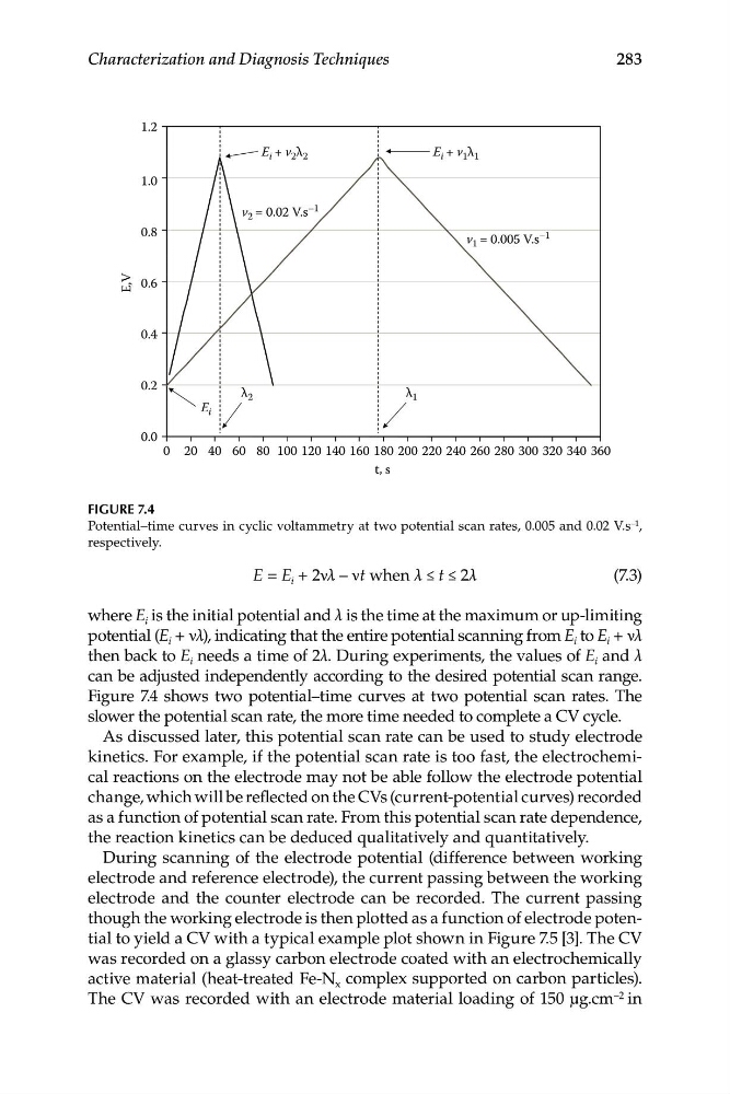
FIGURE 7.4
Potential–time curves in cyclic voltammetry at two potential scan rates, 0.005 and 0.02 V.s –1 ,
respectively.
E = E i + 2νλ – νt when λ ≤ t ≤ 2λ
(7.3)
where E i is the initial potential and λ is the time at the maximum or up-limiting
potential (E i + νλ), indicating that the entire potential scanning from E i to E i + νλ
then back to E i needs a time of 2λ. During experiments, the values of E i and λ
can be adjusted independently according to the desired potential scan range.
Figure 7.4 shows two potential–time curves at two potential scan rates. The
slower the potential scan rate, the more time needed to complete a CV cycle.
As discussed later, this potential scan rate can be used to study electrode
kinetics. For example, if the potential scan rate is too fast, the electrochemical reactions on the electrode may not be able follow the electrode potential
change, which will be reflected on the CVs (current-potential curves) recorded
as a function of potential scan rate. From this potential scan rate dependence,
the reaction kinetics can be deduced qualitatively and quantitatively.
During scanning of the electrode potential (difference between working
electrode and reference electrode), the current passing between the working
electrode and the counter electrode can be recorded. The current passing
though the working electrode is then plotted as a function of electrode potential to yield a CV with a typical example plot shown in Figure 7.5 [3]. The CV
was recorded on a glassy carbon electrode coated with an electrochemically
active material (heat-treated Fe-N x complex supported on carbon particles).
The CV was recorded with an electrode material loading of 150 μg.cm –2 in
1.2
1.0
0.8
0.6
0.4
0.2
0.0
E i + v 2 λ 2
E i + v 1 λ 1
v 2 = 0.02 V.s
–1
v 1 = 0.005 V.s
–1
E i
λ 2
λ 1
0 20 40 60 80 100 120 140 160 180 200 220 240 260 280 300 320 340 360
t, s
283
Characterization and Diagnosis Techniques
FIGURE 7.4
Potential–time curves in cyclic voltammetry at two potential scan rates, 0.005 and 0.02 V.s –1 ,
respectively.
E = E i + 2νλ – νt when λ ≤ t ≤ 2λ
(7.3)
where E i is the initial potential and λ is the time at the maximum or up-limiting
potential (E i + νλ), indicating that the entire potential scanning from E i to E i + νλ
then back to E i needs a time of 2λ. During experiments, the values of E i and λ
can be adjusted independently according to the desired potential scan range.
Figure 7.4 shows two potential–time curves at two potential scan rates. The
slower the potential scan rate, the more time needed to complete a CV cycle.
As discussed later, this potential scan rate can be used to study electrode
kinetics. For example, if the potential scan rate is too fast, the electrochemical reactions on the electrode may not be able follow the electrode potential
change, which will be reflected on the CVs (current-potential curves) recorded
as a function of potential scan rate. From this potential scan rate dependence,
the reaction kinetics can be deduced qualitatively and quantitatively.
During scanning of the electrode potential (difference between working
electrode and reference electrode), the current passing between the working
electrode and the counter electrode can be recorded. The current passing
though the working electrode is then plotted as a function of electrode potential to yield a CV with a typical example plot shown in Figure 7.5 [3]. The CV
was recorded on a glassy carbon electrode coated with an electrochemically
active material (heat-treated Fe-N x complex supported on carbon particles).
The CV was recorded with an electrode material loading of 150 μg.cm –2 in