

Solutions to exercises
79
c. Between the points U = −0.5 V and U = −0.4 V, which gives an average
applied potential of −0.45 V, the equation of the line in figure 31 allows
us to calculate log a O
WE
2
.
.
.
.
.
log a
19 70
2
0 4 0 5
3 57
O
WE
2
=
−
−
−
#
.
log a
12 44
O
WE
2
= −
Furthermore, the electronic conductivity is calculated by applying the
relation
(a )
2 a
1
dU
dI
e O
WE
2
σ
π
=
#
and averaging two successive values of current and potential to calculate the derivative. For example, by using the two pairs (−4.8/−0.4) and
(−11/−0.5), we obtain
(a )
2 170 10
1
( 0.4 0.5)
( 4.8 11) 10
e O
WE
4
6
2
σ
π
=
−
+
−
+
−
−
#
#
#
#
(a ) 5.80 10 S cm
e O
WE
4
1
2
σ
=
−
−
#
or
log (a )
3.24 S cm
e O
WE
1
2
σ
= −
−
The results for log a O
WE
2
and log (a )
e O
WE
2
σ
for each average potential U ave
appear in table 20.
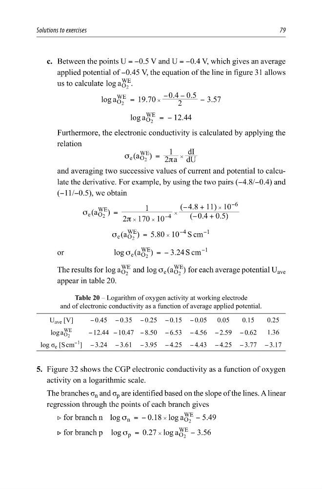
Table 20 – Logarithm of oxygen activity at working electrode
and of electronic conductivity as a function of average applied potential.
U ave [V]
− 0.45 − 0.35 − 0.25 − 0.15 − 0.05 0.05
0.15
0.25
log a O
WE
2
− 12.44 − 10.47 − 8.50 − 6.53 − 4.56 − 2.59 − 0.62 1.36
log σ e [S cm
−1
] − 3.24 − 3.61 − 3.95 − 4.25 − 4.43 − 4.25 − 3.77 − 3.17
5. Figure 32 shows the CGP electronic conductivity as a function of oxygen
activity on a logarithmic scale.
The branches σ n and σ p are identified based on the slope of the lines. A linear
regression through the points of each branch gives
2 for branch n log
0.18 log a
5.49
n
O
WE
2
σ = −
−
#
2 for branch p log
0.27 log a
3.56
p
O
WE
2
σ =
−
#
79
c. Between the points U = −0.5 V and U = −0.4 V, which gives an average
applied potential of −0.45 V, the equation of the line in figure 31 allows
us to calculate log a O
WE
2
.
.
.
.
.
log a
19 70
2
0 4 0 5
3 57
O
WE
2
=
−
−
−
#
.
log a
12 44
O
WE
2
= −
Furthermore, the electronic conductivity is calculated by applying the
relation
(a )
2 a
1
dU
dI
e O
WE
2
σ
π
=
#
and averaging two successive values of current and potential to calculate the derivative. For example, by using the two pairs (−4.8/−0.4) and
(−11/−0.5), we obtain
(a )
2 170 10
1
( 0.4 0.5)
( 4.8 11) 10
e O
WE
4
6
2
σ
π
=
−
+
−
+
−
−
#
#
#
#
(a ) 5.80 10 S cm
e O
WE
4
1
2
σ
=
−
−
#
or
log (a )
3.24 S cm
e O
WE
1
2
σ
= −
−
The results for log a O
WE
2
and log (a )
e O
WE
2
σ
for each average potential U ave
appear in table 20.
Table 20 – Logarithm of oxygen activity at working electrode
and of electronic conductivity as a function of average applied potential.
U ave [V]
− 0.45 − 0.35 − 0.25 − 0.15 − 0.05 0.05
0.15
0.25
log a O
WE
2
− 12.44 − 10.47 − 8.50 − 6.53 − 4.56 − 2.59 − 0.62 1.36
log σ e [S cm
−1
] − 3.24 − 3.61 − 3.95 − 4.25 − 4.43 − 4.25 − 3.77 − 3.17
5. Figure 32 shows the CGP electronic conductivity as a function of oxygen
activity on a logarithmic scale.
The branches σ n and σ p are identified based on the slope of the lines. A linear
regression through the points of each branch gives
2 for branch n log
0.18 log a
5.49
n
O
WE
2
σ = −
−
#
2 for branch p log
0.27 log a
3.56
p
O
WE
2
σ =
−
#