

78
2 – Methods and techniques
with
(
° )
.
a
C
750
2 68 10
O
RE
4
2
=
−
#
For U = − 0.5 V a
e
268 10
O
WE
4 .
(
)
( . )
2
8 314 750 273
4
05 96480
=
−
#
#
#
#
+
−
.
a
376 10
O
WE
14
2
=
−
#
and
.
log a
13 42
O
WE
2
= −
The results for log a O
WE
2
are presented in table 19.
Table 19 – Oxygen activity at working electrode as a function of applied potential.
U [V]
− 0.5
− 0.4
− 0.3
− 0.2
− 0.1
0
0.1
0.2
0.3
log a O
WE
2
− 13.42 − 11.45 − 9.48 − 7.51 − 5.54 − 3.57 − 1.60 0.37
2.34
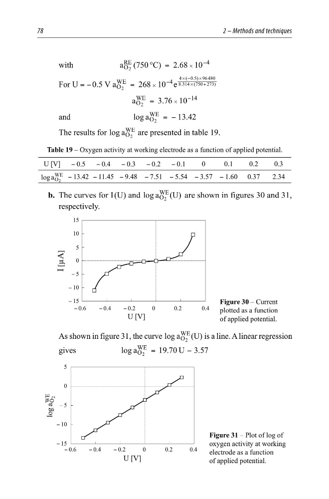
b. The curves for I (U) and
( )
log a
U
O
WE
2
are shown in figures 30 and 31,
respectively.
Figure 30 – Current
plotted as a function
of applied potential.
As shown in figure 31, the curve
( )
log a
U
O
WE
2
is a line. A linear regression
gives
.
.
log a
U
19 70
3 57
O
WE
2
=
−
Figure 31 – Plot of log of
oxygen activity at working
electrode as a function
of applied potential.
<
<
<
<
,>$@
8>9@
<
<
<
<
±
<
<
<
8>9@
ORJ D
2
:(
2 – Methods and techniques
with
(
° )
.
a
C
750
2 68 10
O
RE
4
2
=
−
#
For U = − 0.5 V a
e
268 10
O
WE
4 .
(
)
( . )
2
8 314 750 273
4
05 96480
=
−
#
#
#
#
+
−
.
a
376 10
O
WE
14
2
=
−
#
and
.
log a
13 42
O
WE
2
= −
The results for log a O
WE
2
are presented in table 19.
Table 19 – Oxygen activity at working electrode as a function of applied potential.
U [V]
− 0.5
− 0.4
− 0.3
− 0.2
− 0.1
0
0.1
0.2
0.3
log a O
WE
2
− 13.42 − 11.45 − 9.48 − 7.51 − 5.54 − 3.57 − 1.60 0.37
2.34
b. The curves for I (U) and
( )
log a
U
O
WE
2
are shown in figures 30 and 31,
respectively.
Figure 30 – Current
plotted as a function
of applied potential.
As shown in figure 31, the curve
( )
log a
U
O
WE
2
is a line. A linear regression
gives
.
.
log a
U
19 70
3 57
O
WE
2
=
−
Figure 31 – Plot of log of
oxygen activity at working
electrode as a function
of applied potential.
<
<
<
<
,>$@
8>9@
<
<
<
<
±
<
<
<
8>9@
ORJ D
2
:(