

Course notes
13
1.3.3 – Diagram for MX 2 crystal
The diagram is obtained by plotting in logarithmic coordinates the variation
in concentration of each species as a function of partial pressure P X 2 and at a
given temperature. We can distinguish two cases: K AF & K e and K e & K AF .
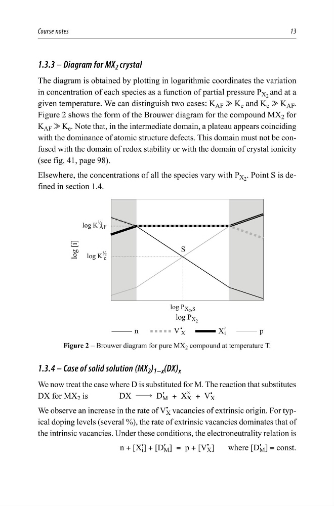
Figure 2 shows the form of the Brouwer diagram for the compound MX 2 for
K AF & K e . Note that, in the intermediate domain, a plateau appears coinciding
with the dominance of atomic structure defects. This domain must not be confused with the domain of redox stability or with the domain of crystal ionicity
(see fig. 41, page 98).
Elsewhere, the concentrations of all the species vary with P X 2 . Point S is defined in section 1.4.
ORJ3 ; 6
Q
9
;
S
6
ORJ.
ò
$)
ORJ.
ò
H
ORJ>L@
ORJ3 ;
; L
l
Figure 2 – Brouwer diagram for pure MX 2 compound at temperature T.
1.3.4 – Case of solid solution (MX 2 ) 1−x (DX) x
We now treat the case where D is substituted for M. The reaction that substitutes
DX for MX 2 is
DX $ D ′
M + X
#
X + V
•
X
We observe an increase in the rate of V
•
X vacancies of extrinsic origin. For typical doping levels (several %), the rate of extrinsic vacancies dominates that of
the intrinsic vacancies. Under these conditions, the electroneutrality relation is
n + [X ′
i ] + [D ′
M ] = p + [V
•
X ]
where [D ′
M ] = const.
13
1.3.3 – Diagram for MX 2 crystal
The diagram is obtained by plotting in logarithmic coordinates the variation
in concentration of each species as a function of partial pressure P X 2 and at a
given temperature. We can distinguish two cases: K AF & K e and K e & K AF .
Figure 2 shows the form of the Brouwer diagram for the compound MX 2 for
K AF & K e . Note that, in the intermediate domain, a plateau appears coinciding
with the dominance of atomic structure defects. This domain must not be confused with the domain of redox stability or with the domain of crystal ionicity
(see fig. 41, page 98).
Elsewhere, the concentrations of all the species vary with P X 2 . Point S is defined in section 1.4.
ORJ3 ; 6
Q
9
;
S
6
ORJ.
ò
$)
ORJ.
ò
H
ORJ>L@
ORJ3 ;
; L
l
Figure 2 – Brouwer diagram for pure MX 2 compound at temperature T.
1.3.4 – Case of solid solution (MX 2 ) 1−x (DX) x
We now treat the case where D is substituted for M. The reaction that substitutes
DX for MX 2 is
DX $ D ′
M + X
#
X + V
•
X
We observe an increase in the rate of V
•
X vacancies of extrinsic origin. For typical doping levels (several %), the rate of extrinsic vacancies dominates that of
the intrinsic vacancies. Under these conditions, the electroneutrality relation is
n + [X ′
i ] + [D ′
M ] = p + [V
•
X ]
where [D ′
M ] = const.