

Solutions to exercises
245
ǻ(
ij
ij
ij
ij
ij
ij
ij
ij
ij
&X $J $J
SRURXV 2
<
<6= 3W2 &X
DOXPLQD VDOW
LQWUHI
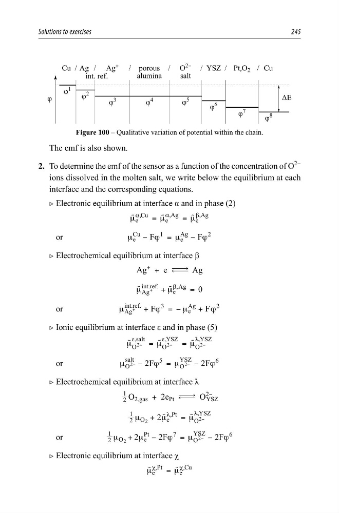
Figure 100 – Qualitative variation of potential within the chain.
The emf is also shown.
2. To determine the emf of the sensor as a function of the concentration of O
2−
ions dissolved in the molten salt, we write below the equilibrium at each
interface and the corresponding equations.
2 Electronic equilibrium at interface α and in phase (2)
e
,Cu
e
,Ag
e
,Ag
μ
μ
μ
=
=
α
α
β
u
u
u
or
F
F
e
Cu
1
e
Ag
2
μ
ϕ
μ
ϕ
−
=
−
2 Electrochemical equilibrium at interface β
Ag
+ + e m Ag
0
Ag
int.ref.
e
,Ag
μ
μ
+
=
β
+
u
u
or
F
F
Ag
int.ref.
3
e
Ag
2
μ
ϕ
μ
ϕ
+
= −
+
+
2 Ionic equilibrium at interface ε and in phase (5)
O
,salt
O
,YSZ
O
,YSZ
2
2
2
μ
μ
μ
=
=
ε
ε
λ
−
−
−
u
u
u
or
2F
2F
O
salt
5
O
YSZ
6
2
2
μ
ϕ
μ
ϕ
−
=
−
−
−
2 Electrochemical equilibrium at interface λ
2
1
O 2,gas + 2e Pt m O
2−
YSZ
2
2
1 O
e
,Pt
O
,YSZ
2
2
μ
μ
μ
+
=
λ
λ
−
u
u
or
2
2F
2 F
2
1 O
e
Pt
7
O
YSZ
6
2
2
μ
μ
ϕ
μ
ϕ
+
−
=
−
−
2 Electronic equilibrium at interface χ
e
,Pt
e
,Cu
μ
μ
=
χ
χ
u
u
245
ǻ(
ij
ij
ij
ij
ij
ij
ij
ij
ij
&X $J $J
SRURXV 2
<
<6= 3W2 &X
DOXPLQD VDOW
LQWUHI
Figure 100 – Qualitative variation of potential within the chain.
The emf is also shown.
2. To determine the emf of the sensor as a function of the concentration of O
2−
ions dissolved in the molten salt, we write below the equilibrium at each
interface and the corresponding equations.
2 Electronic equilibrium at interface α and in phase (2)
e
,Cu
e
,Ag
e
,Ag
μ
μ
μ
=
=
α
α
β
u
u
u
or
F
F
e
Cu
1
e
Ag
2
μ
ϕ
μ
ϕ
−
=
−
2 Electrochemical equilibrium at interface β
Ag
+ + e m Ag
0
Ag
int.ref.
e
,Ag
μ
μ
+
=
β
+
u
u
or
F
F
Ag
int.ref.
3
e
Ag
2
μ
ϕ
μ
ϕ
+
= −
+
+
2 Ionic equilibrium at interface ε and in phase (5)
O
,salt
O
,YSZ
O
,YSZ
2
2
2
μ
μ
μ
=
=
ε
ε
λ
−
−
−
u
u
u
or
2F
2F
O
salt
5
O
YSZ
6
2
2
μ
ϕ
μ
ϕ
−
=
−
−
−
2 Electrochemical equilibrium at interface λ
2
1
O 2,gas + 2e Pt m O
2−
YSZ
2
2
1 O
e
,Pt
O
,YSZ
2
2
μ
μ
μ
+
=
λ
λ
−
u
u
or
2
2F
2 F
2
1 O
e
Pt
7
O
YSZ
6
2
2
μ
μ
ϕ
μ
ϕ
+
−
=
−
−
2 Electronic equilibrium at interface χ
e
,Pt
e
,Cu
μ
μ
=
χ
χ
u
u