

Exercises
105
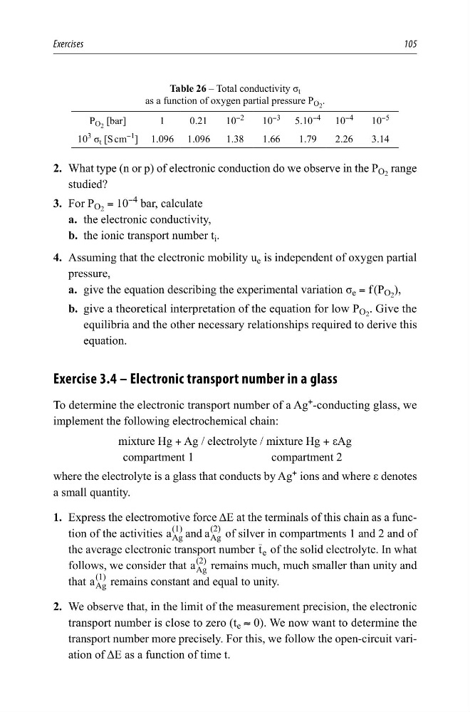
Table 26 – Total conductivity σ t
as a function of oxygen partial pressure P O 2 .
P O 2 [bar]
1
0.21
10
−2
10
−3
5.10
−4
10
−4
10
−5
10
3
σ t [S cm
−1
] 1.096 1.096
1.38
1.66
1.79
2.26
3.14
2. What type (n or p) of electronic conduction do we observe in the P O 2 range
studied?
3. For P O 2 = 10
−4
bar, calculate
a. the electronic conductivity,
b. the ionic transport number t i .
4. Assuming that the electronic mobility u e is independent of oxygen partial
pressure,
a. give the equation describing the experimental variation σ e = f (P O 2 ),
b. give a theoretical interpretation of the equation for low P O 2 . Give the
equilibria and the other necessary relationships required to derive this
equation.
Exercise 3.4 – Electronic transport number in a glass
To determine the electronic transport number of a Ag
+
-conducting glass, we
implement the following electrochemical chain:
mixture Hg + Ag / electrolyte / mixture Hg + εAg
compartment 1
compartment 2
where the electrolyte is a glass that conducts by Ag
+
ions and where ε denotes
a small quantity.
1. Express the electromotive force ΔE at the terminals of this chain as a function of the activities a and a
( )
( )
Ag
Ag
1
2
of silver in compartments 1 and 2 and of
the average electronic transport number t e
r of the solid electrolyte. In what
follows, we consider that a
( )
Ag
2
remains much, much smaller than unity and
that a
( )
Ag
1
remains constant and equal to unity.
2. We observe that, in the limit of the measurement precision, the electronic
transport number is close to zero (t e ≈ 0). We now want to determine the
transport number more precisely. For this, we follow the open-circuit variation of ΔE as a function of time t.
105
Table 26 – Total conductivity σ t
as a function of oxygen partial pressure P O 2 .
P O 2 [bar]
1
0.21
10
−2
10
−3
5.10
−4
10
−4
10
−5
10
3
σ t [S cm
−1
] 1.096 1.096
1.38
1.66
1.79
2.26
3.14
2. What type (n or p) of electronic conduction do we observe in the P O 2 range
studied?
3. For P O 2 = 10
−4
bar, calculate
a. the electronic conductivity,
b. the ionic transport number t i .
4. Assuming that the electronic mobility u e is independent of oxygen partial
pressure,
a. give the equation describing the experimental variation σ e = f (P O 2 ),
b. give a theoretical interpretation of the equation for low P O 2 . Give the
equilibria and the other necessary relationships required to derive this
equation.
Exercise 3.4 – Electronic transport number in a glass
To determine the electronic transport number of a Ag
+
-conducting glass, we
implement the following electrochemical chain:
mixture Hg + Ag / electrolyte / mixture Hg + εAg
compartment 1
compartment 2
where the electrolyte is a glass that conducts by Ag
+
ions and where ε denotes
a small quantity.
1. Express the electromotive force ΔE at the terminals of this chain as a function of the activities a and a
( )
( )
Ag
Ag
1
2
of silver in compartments 1 and 2 and of
the average electronic transport number t e
r of the solid electrolyte. In what
follows, we consider that a
( )
Ag
2
remains much, much smaller than unity and
that a
( )
Ag
1
remains constant and equal to unity.
2. We observe that, in the limit of the measurement precision, the electronic
transport number is close to zero (t e ≈ 0). We now want to determine the
transport number more precisely. For this, we follow the open-circuit variation of ΔE as a function of time t.