

86
2 – Methods and techniques
Table 22 – Cationic conductivity of CaF 2 as a function of temperature.
T [°C]
632
718
798
864
σ c [S cm
−1
] 1.65 # 10
−12
9.72 # 10
−12
5.28 # 10
−11
1.44 # 10
−10
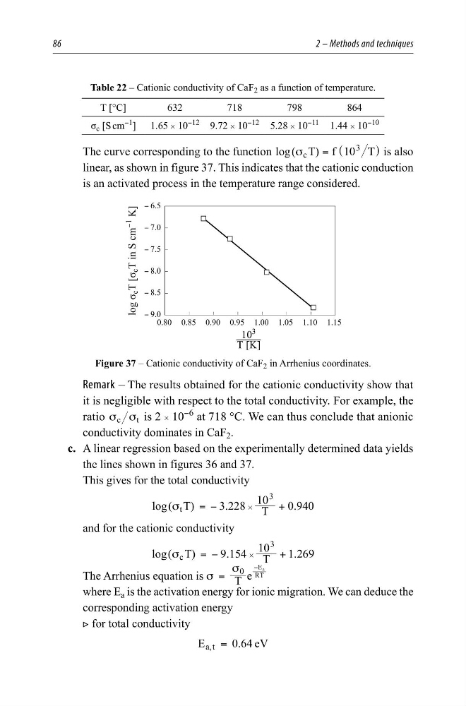
The curve corresponding to the function log( T) f 10 T
c
3
σ
= ^
h is also
linear, as shown in figure 37. This indicates that the cationic conduction
is an activated process in the temperature range considered.
—
7>.@
ORJı
F 7>ı
F 7LQ6FP
<
.@
<
<
<
<
<
<
Figure 37 – Cationic conductivity of CaF 2 in Arrhenius coordinates.
Remark – The results obtained for the cationic conductivity show that
it is negligible with respect to the total conductivity. For example, the
ratio c t
σ σ is 2 # 10
−6
at 718 °C. We can thus conclude that anionic
conductivity dominates in CaF 2 .
c. A linear regression based on the experimentally determined data yields
the lines shown in figures 36 and 37.
This gives for the total conductivity
log( T)
3.228 T
10
0.940
t
3
σ
= −
+
#
and for the cationic conductivity
log( T)
9.154 T
10
1.269
c
3
σ
= −
+
#
The Arrhenius equation is
T e
0 RT
E a
σ
σ
=
−
where E a is the activation energy for ionic migration. We can deduce the
corresponding activation energy
2 for total conductivity
.
E
e V
0 64
,
a t =
2 – Methods and techniques
Table 22 – Cationic conductivity of CaF 2 as a function of temperature.
T [°C]
632
718
798
864
σ c [S cm
−1
] 1.65 # 10
−12
9.72 # 10
−12
5.28 # 10
−11
1.44 # 10
−10
The curve corresponding to the function log( T) f 10 T
c
3
σ
= ^
h is also
linear, as shown in figure 37. This indicates that the cationic conduction
is an activated process in the temperature range considered.
—
7>.@
ORJı
F 7>ı
F 7LQ6FP
<
.@
<
<
<
<
<
<
Figure 37 – Cationic conductivity of CaF 2 in Arrhenius coordinates.
Remark – The results obtained for the cationic conductivity show that
it is negligible with respect to the total conductivity. For example, the
ratio c t
σ σ is 2 # 10
−6
at 718 °C. We can thus conclude that anionic
conductivity dominates in CaF 2 .
c. A linear regression based on the experimentally determined data yields
the lines shown in figures 36 and 37.
This gives for the total conductivity
log( T)
3.228 T
10
0.940
t
3
σ
= −
+
#
and for the cationic conductivity
log( T)
9.154 T
10
1.269
c
3
σ
= −
+
#
The Arrhenius equation is
T e
0 RT
E a
σ
σ
=
−
where E a is the activation energy for ionic migration. We can deduce the
corresponding activation energy
2 for total conductivity
.
E
e V
0 64
,
a t =