

74
Chapter 2. Geometrical optics
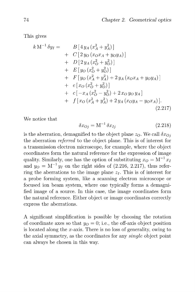
This gives
k M
−1 δy I =
2
A ) ]
B [ 4 y A (x
2
A + y
+ C [ 2 y O (x O x A + y O y A ) ]
D [ 2 y A (x O + y
2
2
O ) ]
+
E [ y O (x O + y
2
O ) ]
2
2
+
F [ y O (x A + y
2
) + 2 y A (x O x A + y O y A ) ]
+
A
e [ x O (x O + y
2
2
O ) ]
2
+
c [ −x A (x
2
O
2
− y O ) + 2 x O y O y A ]
A ) + 2 y A (x O y A − y O x A ) ].
+
2 + y
A
+ f [ x O (x
(2.217)
We notice that
δx Oj = M
−1 δx Ij
(2.218)
is the aberration, demagnified to the object plane z O . We call δx Oj
the aberration referred to the object plane. This is of interest for
a transmission electron microscope, for example, where the object
coordinates form the natural reference for the expression of image
quality. Similarly, one has the option of substituting x O = M
−1 x I
and y
1
O = M
− y I on the right sides of (2.216, 2.217), thus referring the aberrations to the image plane z I . This is of interest for
a probe forming system, like a scanning electron microscope or
focused ion beam system, where one typically forms a demagnified image of a source. In this case, the image coordinates form
the natural reference. Either object or image coordinates correctly
express the aberrations.
A significant simplification is possible by choosing the rotation
of coordinate axes so that y O = 0; i.e., the off-axis object position
is located along the x-axis. There is no loss of generality, owing to
the axial symmetry, as the coordinates for any single object point
can always be chosen in this way.
Chapter 2. Geometrical optics
This gives
k M
−1 δy I =
2
A ) ]
B [ 4 y A (x
2
A + y
+ C [ 2 y O (x O x A + y O y A ) ]
D [ 2 y A (x O + y
2
2
O ) ]
+
E [ y O (x O + y
2
O ) ]
2
2
+
F [ y O (x A + y
2
) + 2 y A (x O x A + y O y A ) ]
+
A
e [ x O (x O + y
2
2
O ) ]
2
+
c [ −x A (x
2
O
2
− y O ) + 2 x O y O y A ]
A ) + 2 y A (x O y A − y O x A ) ].
+
2 + y
A
+ f [ x O (x
(2.217)
We notice that
δx Oj = M
−1 δx Ij
(2.218)
is the aberration, demagnified to the object plane z O . We call δx Oj
the aberration referred to the object plane. This is of interest for
a transmission electron microscope, for example, where the object
coordinates form the natural reference for the expression of image
quality. Similarly, one has the option of substituting x O = M
−1 x I
and y
1
O = M
− y I on the right sides of (2.216, 2.217), thus referring the aberrations to the image plane z I . This is of interest for
a probe forming system, like a scanning electron microscope or
focused ion beam system, where one typically forms a demagnified image of a source. In this case, the image coordinates form
the natural reference. Either object or image coordinates correctly
express the aberrations.
A significant simplification is possible by choosing the rotation
of coordinate axes so that y O = 0; i.e., the off-axis object position
is located along the x-axis. There is no loss of generality, owing to
the axial symmetry, as the coordinates for any single object point
can always be chosen in this way.