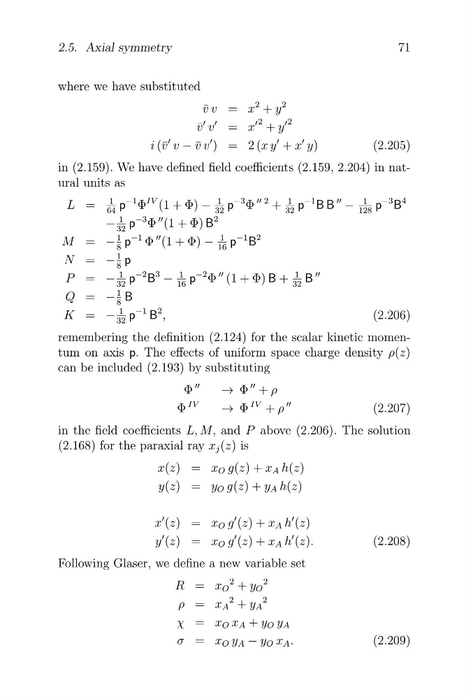
�
�
�
where we have substituted
¯ =
2 + y
2
v v
x
� �
� 2
� 2
v ¯ v = x + y
i (¯ v
v v = 2 (x y + x y)
(2.205)
v − ¯
� )
in (2.159). We have defined field coefficients (2.159, 2.204) in natural units as
1
1 −3 Φ
�� 2
1
1
−3 B
4
L =
p
−1 Φ
IV (1 + Φ) − p
+ p
−1 B B
�� −
p
64
32
32
128
−
1 p
−3 Φ
�� (1 + Φ) B
2
32

1 −1 B
2

M = −
1
8
p
−1 Φ
�� (1 + Φ) − 16 p

−
1

N =
8
p

−
1 −2 B
3 −
1
1 B
��

P =
p
p
−2 Φ
�� (1 + Φ) B +
32
16
32

−
1

Q =
8
B

K = −
1 p
−1 B
2 ,
(2.206)

32
remembering the definition (2.124) for the scalar kinetic momentum on axis p. The effects of uniform space charge density ρ(z)
can be included (2.193) by substituting
Φ
��
→ Φ
�� + ρ
Φ
IV
→ Φ
IV + ρ
��
(2.207)
in the field coefficients L, M, and P above (2.206). The solution
(2.168) for the paraxial ray x j (z) is
x(z) = x O g(z) + x A h(z)
y(z) = y O g(z) + y A h(z)
x
� (z) = x O g
� (z) + x A h
� (z)
y
� (z) = x O g
� (z) + x A h
� (z).
(2.208)
Following Glaser, we define a new variable set
R = x O
2 + y O
2
ρ = x A
2 + y A
2
χ = x O x A + y O y A
σ = x O y A − y O x A .
(2.209)
71
2.5. Axial symmetry