

� �
�
�
�
� �
�
�
�
� �
�
�
�
62
Chapter 2. Geometrical optics
From (2.160, 2.170) we obtain
1 � �
m 2 =
w ¯ w
2
+ −
1 p
−2 Φ
�� (1 + Φ) +
1 p
−4 Φ
� 2 (1 + Φ)
2 −
1 p
−2 B
2 ww ¯
4
8
8
−
1
�
� ).
4
p
−2 Φ
� (1 + Φ) ( ¯
w w + ww ¯
(2.171)
From (2.104) we have
∂m 2
d ∂m 2
−
�
= 0.
(2.172)
∂w ¯
dz ∂w ¯
This yields the paraxial ray equation in reduced coordinates as
follows:
d
2 w
3
−2 Φ
� 2
1 −2 B
2
+ p
−4 Φ
� 2 (1 + Φ)
2 −
1 p
+ p
w = 0, (2.173)
4
2
4
dz 2
where the second-order derivative Φ
�� has been successfully eliminated. Although the reduced ray w(z) offers a practical simplification for obtaining the paraxial ray solution numerically, it offers
no advantage for obtaining the aberrations.
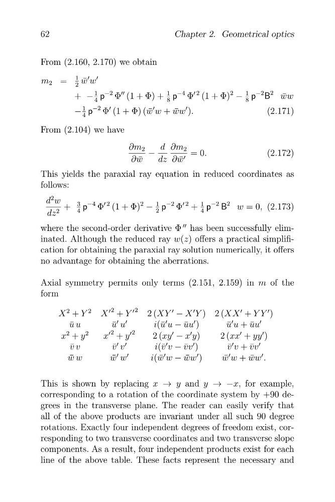
Axial symmetry permits only terms (2.151, 2.159) in m of the
form
X
2 + Y
2
X
� 2 + Y
� 2
2 (XY
� − X
� Y ) 2 (XX
� + Y Y
� )
u u
¯
¯ u
u
uu
¯ u + ¯
u
i(¯ u − ¯
� )
u
uu
2
� 2
� 2
�
x
2 + y
x + y
2 (xy
� − x y)
2 (xx
� + yy
� )
¯
¯ v
v
vv
� )
v
vv
v v
v
i(¯ v − ¯
¯ v + ¯
w w
¯
¯ w
w w − ¯
� )
¯ w + ww
w
i( ¯
ww
w
¯ .
This is shown by replacing x → y and y → −x, for example,
corresponding to a rotation of the coordinate system by +90 degrees in the transverse plane. The reader can easily verify that
all of the above products are invariant under all such 90 degree
rotations. Exactly four independent degrees of freedom exist, corresponding to two transverse coordinates and two transverse slope
components. As a result, four independent products exist for each
line of the above table. These facts represent the necessary and
�
�
�
� �
�
�
�
� �
�
�
�
62
Chapter 2. Geometrical optics
From (2.160, 2.170) we obtain
1 � �
m 2 =
w ¯ w
2
+ −
1 p
−2 Φ
�� (1 + Φ) +
1 p
−4 Φ
� 2 (1 + Φ)
2 −
1 p
−2 B
2 ww ¯
4
8
8
−
1
�
� ).
4
p
−2 Φ
� (1 + Φ) ( ¯
w w + ww ¯
(2.171)
From (2.104) we have
∂m 2
d ∂m 2
−
�
= 0.
(2.172)
∂w ¯
dz ∂w ¯
This yields the paraxial ray equation in reduced coordinates as
follows:
d
2 w
3
−2 Φ
� 2
1 −2 B
2
+ p
−4 Φ
� 2 (1 + Φ)
2 −
1 p
+ p
w = 0, (2.173)
4
2
4
dz 2
where the second-order derivative Φ
�� has been successfully eliminated. Although the reduced ray w(z) offers a practical simplification for obtaining the paraxial ray solution numerically, it offers
no advantage for obtaining the aberrations.
Axial symmetry permits only terms (2.151, 2.159) in m of the
form
X
2 + Y
2
X
� 2 + Y
� 2
2 (XY
� − X
� Y ) 2 (XX
� + Y Y
� )
u u
¯
¯ u
u
uu
¯ u + ¯
u
i(¯ u − ¯
� )
u
uu
2
� 2
� 2
�
x
2 + y
x + y
2 (xy
� − x y)
2 (xx
� + yy
� )
¯
¯ v
v
vv
� )
v
vv
v v
v
i(¯ v − ¯
¯ v + ¯
w w
¯
¯ w
w w − ¯
� )
¯ w + ww
w
i( ¯
ww
w
¯ .
This is shown by replacing x → y and y → −x, for example,
corresponding to a rotation of the coordinate system by +90 degrees in the transverse plane. The reader can easily verify that
all of the above products are invariant under all such 90 degree
rotations. Exactly four independent degrees of freedom exist, corresponding to two transverse coordinates and two transverse slope
components. As a result, four independent products exist for each
line of the above table. These facts represent the necessary and