

�
� �
�
�
�
42
Chapter 2. Geometrical optics
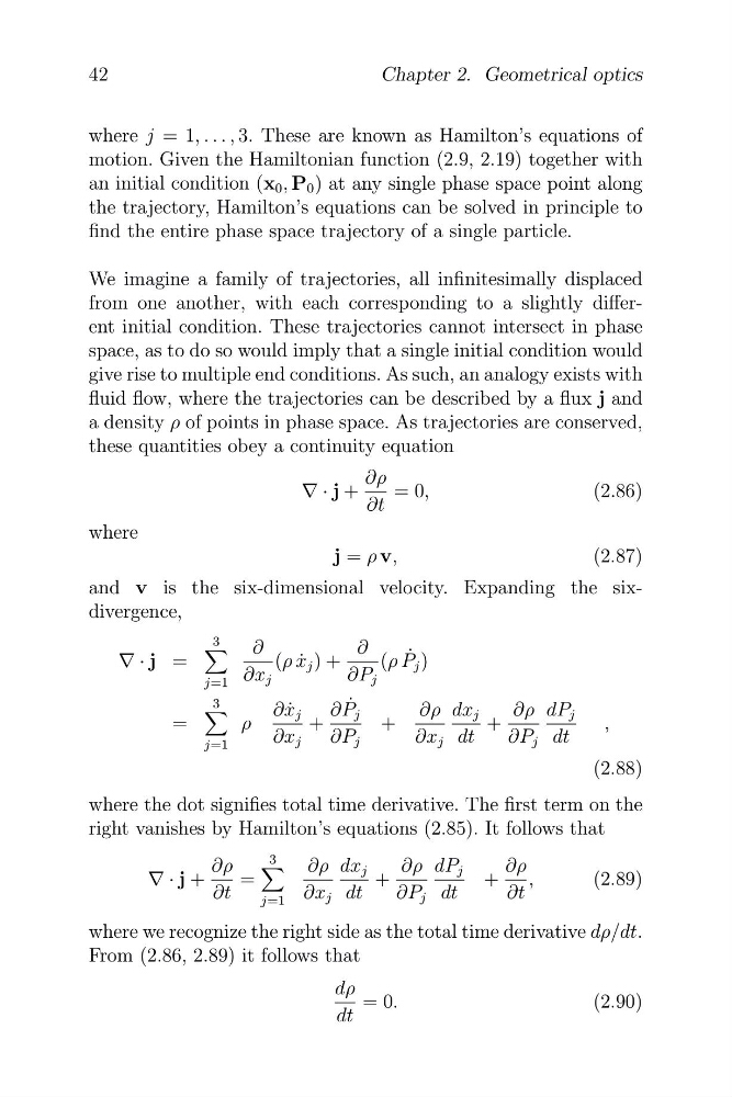
where j = 1, . . . , 3. These are known as Hamilton’s equations of
motion. Given the Hamiltonian function (2.9, 2.19) together with
an initial condition (x 0 , P 0 ) at any single phase space point along
the trajectory, Hamilton’s equations can be solved in principle to
find the entire phase space trajectory of a single particle.
We imagine a family of trajectories, all infinitesimally displaced
from one another, with each corresponding to a slightly different initial condition. These trajectories cannot intersect in phase
space, as to do so would imply that a single initial condition would
give rise to multiple end conditions. As such, an analogy exists with
fluid flow, where the trajectories can be described by a flux j and
a density ρ of points in phase space. As trajectories are conserved,
these quantities obey a continuity equation
∂ρ
v · j +
= 0,
(2.86)
∂t
where
j = ρ v,
(2.87)
and v is the six-dimensional velocity. Expanding the sixdivergence,
3
4
v · j =
∂ (ρ x ˙ j ) +
∂ (ρ P ˙ j )
j=1 ∂x j
∂P j
3
4
∂x ˙ j ∂P ˙ j
∂ρ dx j
∂ρ dP j
=
ρ
+
+
+
,
j=1
∂x j ∂P j
∂x j dt
∂P j dt
(2.88)
where the dot signifies total time derivative. The first term on the
right vanishes by Hamilton’s equations (2.85). It follows that
3
∂ρ 4 ∂ρ dx j
∂ρ dP j
∂ρ
v · j +
=
+
+ ,
(2.89)
∂t j=1 ∂x j dt
∂P j dt
∂t
where we recognize the right side as the total time derivative dρ/dt.
From (2.86, 2.89) it follows that
dρ = 0.
(2.90)
dt
� �
�
�
�
42
Chapter 2. Geometrical optics
where j = 1, . . . , 3. These are known as Hamilton’s equations of
motion. Given the Hamiltonian function (2.9, 2.19) together with
an initial condition (x 0 , P 0 ) at any single phase space point along
the trajectory, Hamilton’s equations can be solved in principle to
find the entire phase space trajectory of a single particle.
We imagine a family of trajectories, all infinitesimally displaced
from one another, with each corresponding to a slightly different initial condition. These trajectories cannot intersect in phase
space, as to do so would imply that a single initial condition would
give rise to multiple end conditions. As such, an analogy exists with
fluid flow, where the trajectories can be described by a flux j and
a density ρ of points in phase space. As trajectories are conserved,
these quantities obey a continuity equation
∂ρ
v · j +
= 0,
(2.86)
∂t
where
j = ρ v,
(2.87)
and v is the six-dimensional velocity. Expanding the sixdivergence,
3
4
v · j =
∂ (ρ x ˙ j ) +
∂ (ρ P ˙ j )
j=1 ∂x j
∂P j
3
4
∂x ˙ j ∂P ˙ j
∂ρ dx j
∂ρ dP j
=
ρ
+
+
+
,
j=1
∂x j ∂P j
∂x j dt
∂P j dt
(2.88)
where the dot signifies total time derivative. The first term on the
right vanishes by Hamilton’s equations (2.85). It follows that
3
∂ρ 4 ∂ρ dx j
∂ρ dP j
∂ρ
v · j +
=
+
+ ,
(2.89)
∂t j=1 ∂x j dt
∂P j dt
∂t
where we recognize the right side as the total time derivative dρ/dt.
From (2.86, 2.89) it follows that
dρ = 0.
(2.90)
dt