

2.3. Conservation laws
37
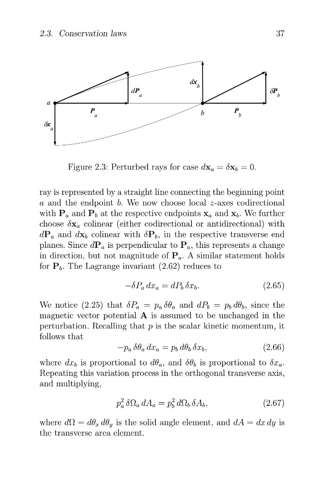
Figure 2.3: Perturbed rays for case dx a = δx b = 0.
ray is represented by a straight line connecting the beginning point
a and the endpoint b. We now choose local z-axes codirectional
with P a and P b at the respective endpoints x a and x b . We further
choose δx a colinear (either codirectional or antidirectional) with
dP a and dx b colinear with δP b , in the respective transverse end
planes. Since dP a is perpendicular to P a , this represents a change
in direction, but not magnitude of P a . A similar statement holds
for P b . The Lagrange invariant (2.62) reduces to
−δP a dx a = dP b δx b .
(2.65)
We notice (2.25) that δP a = p a δθ a and dP b = p b dθ b , since the
magnetic vector potential A is assumed to be unchanged in the
perturbation. Recalling that p is the scalar kinetic momentum, it
follows that
−p a δθ a dx a = p b dθ b δx b ,
(2.66)
where dx b is proportional to dθ a , and δθ b is proportional to δx a .
Repeating this variation process in the orthogonal transverse axis,
and multiplying,
p
2
a δΩ a dA a = p
2
b dΩ b δA b ,
(2.67)
where dΩ = dθ x dθ y is the solid angle element, and dA = dx dy is
the transverse area element.
37
Figure 2.3: Perturbed rays for case dx a = δx b = 0.
ray is represented by a straight line connecting the beginning point
a and the endpoint b. We now choose local z-axes codirectional
with P a and P b at the respective endpoints x a and x b . We further
choose δx a colinear (either codirectional or antidirectional) with
dP a and dx b colinear with δP b , in the respective transverse end
planes. Since dP a is perpendicular to P a , this represents a change
in direction, but not magnitude of P a . A similar statement holds
for P b . The Lagrange invariant (2.62) reduces to
−δP a dx a = dP b δx b .
(2.65)
We notice (2.25) that δP a = p a δθ a and dP b = p b dθ b , since the
magnetic vector potential A is assumed to be unchanged in the
perturbation. Recalling that p is the scalar kinetic momentum, it
follows that
−p a δθ a dx a = p b dθ b δx b ,
(2.66)
where dx b is proportional to dθ a , and δθ b is proportional to δx a .
Repeating this variation process in the orthogonal transverse axis,
and multiplying,
p
2
a δΩ a dA a = p
2
b dΩ b δA b ,
(2.67)
where dΩ = dθ x dθ y is the solid angle element, and dA = dx dy is
the transverse area element.