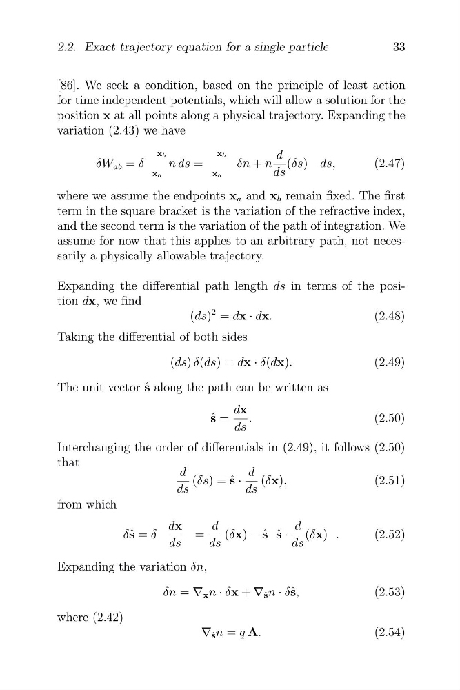
�
�
[86]. We seek a condition, based on the principle of least action
for time independent potentials, which will allow a solution for the
position x at all points along a physical trajectory. Expanding the
variation (2.43) we have
x b
x b
d
δW ab = δ
n ds =
δn + n (δs) ds,
(2.47)
xa
xa
ds
where we assume the endpoints x a and x b remain fixed. The first
term in the square bracket is the variation of the refractive index,
and the second term is the variation of the path of integration. We
assume for now that this applies to an arbitrary path, not necessarily a physically allowable trajectory.
Expanding the differential path length ds in terms of the position dx, we find
(ds)
2 = dx · dx.
(2.48)
Taking the differential of both sides
(ds) δ(ds) = dx · δ(dx).
(2.49)
The unit vector ˆ s along the path can be written as
dx
ˆ s =
.
(2.50)
ds
Interchanging the order of differentials in (2.49), it follows (2.50)
that
d
d
ds
(δs) = ˆ s · ds
(δx),
(2.51)
from which
dx
d
d
δˆ s = δ ds
= ds
(δx) − ˆ s ˆ s · ds
(δx) .
(2.52)
Expanding the variation δn,
δn = v x n · δx + v ˆ s n · δˆ s,
(2.53)
where (2.42)
v ˆ s n = q A.
(2.54)
33
2.2. Exact trajectory equation for a single particle