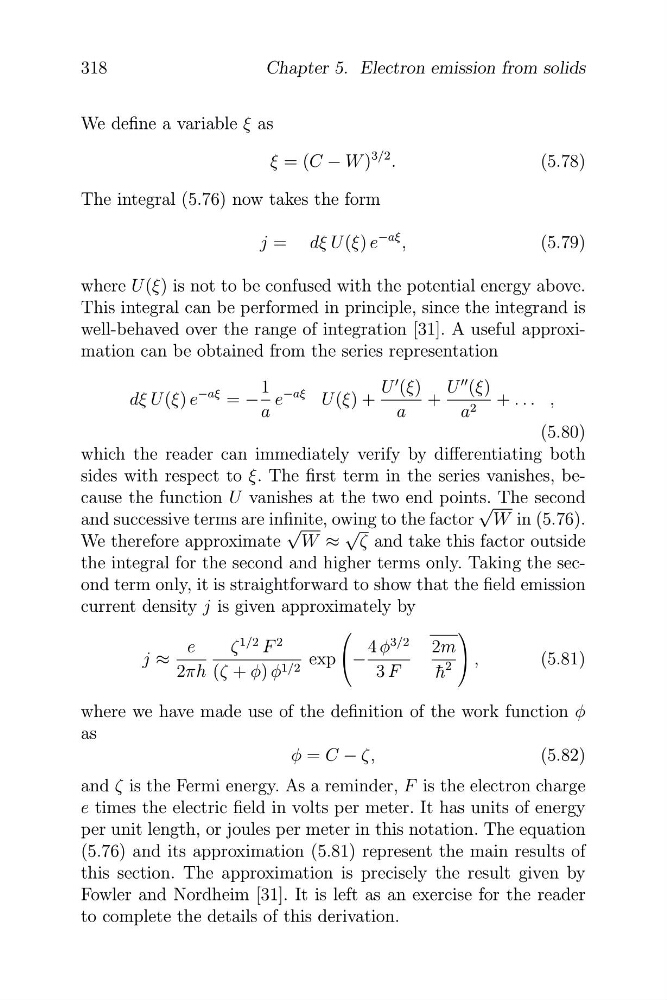
We define a variable ξ as
ξ = (C − W )
3/2 .
(5.78)
The integral (5.76) now takes the form
j = dξ U (ξ) e
−aξ ,
(5.79)
where U (ξ) is not to be confused with the potential energy above.
This integral can be performed in principle, since the integrand is
well-behaved over the range of integration [31]. A useful approximation can be obtained from the series representation
U
�� (ξ)
1
U
� (ξ)
−aξ
−aξ
dξ U (ξ) e
= − e
U (ξ) +
+
+ . . . ,
a
a
a 2
(5.80)
which the reader can immediately verify by differentiating both
sides with respect to ξ. The first term in the series vanishes, because the function U vanishes at the two end points. The second
√
and successive terms are infinite, owing to the factor W in (5.76).
√
√
We therefore approximate W ≈ ζ and take this factor outside
the integral for the second and higher terms only. Taking the second term only, it is straightforward to show that the field emission
current density j is given approximately by
⎛
⎞
ζ
1/2 F
2
4 φ
3/2
e
2m
⎝ −
⎠
j ≈
exp
,
(5.81)
2πh (ζ + φ) φ 1/2
3 F
h ¯
2
where we have made use of the definition of the work function φ
as
φ = C − ζ,
(5.82)
and ζ is the Fermi energy. As a reminder, F is the electron charge
e times the electric field in volts per meter. It has units of energy
per unit length, or joules per meter in this notation. The equation
(5.76) and its approximation (5.81) represent the main results of
this section. The approximation is precisely the result given by
Fowler and Nordheim [31]. It is left as an exercise for the reader
to complete the details of this derivation.
318
Chapter 5. Electron emission from solids