

316
Chapter 5. Electron emission from solids
The fraction of electrons incident on the barrier from within the
bulk, which tunnel through the barrier to be emitted into the
vacuum is given by
j + (x ≥ 0)
D(W ) =
,
(5.69)
j + (x ≤ 0)
where this depends on the energy W . Substituting the above expressions for the two currents, this is
α |b + |
2
D(W ) =
.
(5.70)
πk |a + | 2
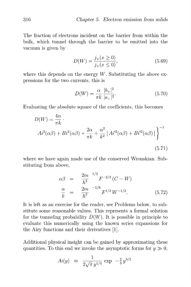
Evaluating the absolute square of the coefficients, this becomes
4α
D(W ) =
·
πk
� −1
2α α
2
Ai
2 (αβ) + Bi
2 (αβ) +
+ k 2 [ Ai
�2 (αβ) + Bi
�2 (αβ) ]
πk
(5.71)
where we have again made use of the conserved Wronskian. Substituting from above,
1/3
αβ =
2m
F
−2/3 (C − W )
h
2
¯
−1/6
α
2m
F
1/3 W
−1/2
=
.
(5.72)
k
h ¯
2
It is left as an exercise for the reader, see Problems below, to substitute some reasonable values. This represents a formal solution
for the tunneling probability D(W ). It is possible in principle to
evaluate this numerically using the known series expansions for
the Airy functions and their derivatives [1].
Additional physical insight can be gained by approximating these
quantities. To this end we invoke the asymptotic forms for y � 0,
1
Ai(y) ≈ √
exp − 3
2 y
3/2
2 π y 1/4
Chapter 5. Electron emission from solids
The fraction of electrons incident on the barrier from within the
bulk, which tunnel through the barrier to be emitted into the
vacuum is given by
j + (x ≥ 0)
D(W ) =
,
(5.69)
j + (x ≤ 0)
where this depends on the energy W . Substituting the above expressions for the two currents, this is
α |b + |
2
D(W ) =
.
(5.70)
πk |a + | 2
Evaluating the absolute square of the coefficients, this becomes
4α
D(W ) =
·
πk
� −1
2α α
2
Ai
2 (αβ) + Bi
2 (αβ) +
+ k 2 [ Ai
�2 (αβ) + Bi
�2 (αβ) ]
πk
(5.71)
where we have again made use of the conserved Wronskian. Substituting from above,
1/3
αβ =
2m
F
−2/3 (C − W )
h
2
¯
−1/6
α
2m
F
1/3 W
−1/2
=
.
(5.72)
k
h ¯
2
It is left as an exercise for the reader, see Problems below, to substitute some reasonable values. This represents a formal solution
for the tunneling probability D(W ). It is possible in principle to
evaluate this numerically using the known series expansions for
the Airy functions and their derivatives [1].
Additional physical insight can be gained by approximating these
quantities. To this end we invoke the asymptotic forms for y � 0,
1
Ai(y) ≈ √
exp − 3
2 y
3/2
2 π y 1/4