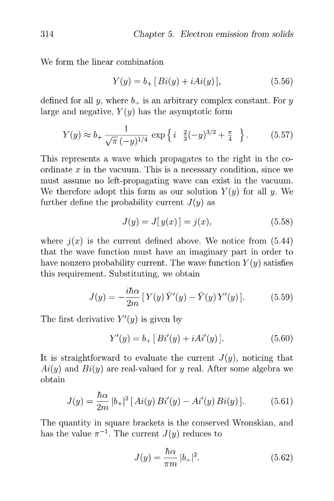
We form the linear combination
Y (y) = b + [ Bi(y) + iAi(y) ],
(5.56)
defined for all y, where b + is an arbitrary complex constant. For y
large and negative, Y (y) has the asymptotic form
1
2 (−y)
3/2
π
Y (y) ≈ b + √
exp i 3
+ 4
.
(5.57)
π (−y) 1/4
This represents a wave which propagates to the right in the coordinate x in the vacuum. This is a necessary condition, since we
must assume no left-propagating wave can exist in the vacuum.
We therefore adopt this form as our solution Y (y) for all y. We
further define the probability current J(y) as
J(y) = J[ y(x) ] = j(x),
(5.58)
where j(x) is the current defined above. We notice from (5.44)
that the wave function must have an imaginary part in order to
have nonzero probability current. The wave function Y (y) satisfies
this requirement. Substituting, we obtain
hα
J(y) = −
i¯ [ Y (y) Y ¯ � (y) − Y ¯ (y) Y
� (y) ].
(5.59)
2m
The first derivative Y
� (y) is given by
Y
� (y) = b + [ Bi
� (y) + iAi
� (y) ].
(5.60)
It is straightforward to evaluate the current J(y), noticing that
Ai(y) and Bi(y) are real-valued for y real. After some algebra we
obtain
¯
hα
J(y) =
|b + |
2 [ Ai(y) Bi
� (y) − Ai
� (y) Bi(y) ].
(5.61)
2m
The quantity in square brackets is the conserved Wronskian, and
has the value π
−1 . The current J(y) reduces to
¯
hα
J(y) =
|b + |
2 .
(5.62)
πm
314
Chapter 5. Electron emission from solids