

which represents two counterpropagating, travelling waves. The
wave number k 1 is given by
2m
k 1 =
W ,
(5.23)
h
2
¯
where we intentionally choose the positive root. In the vacuum
with x ≥ 0 the wave function is
+ik 2 x
u(x ≥ 0) = b + e
,
(5.24)
where the complex constant b + has yet to be determined. The wave
number k 2 is given by
2m
k 2 =
(W − C),
(5.25)
h
2
¯
We assume that no left-propagating wave exists in the vacuum
region x ≥ 0. We need only consider energy W ≥ C, since there
can be no transmission for W < C.
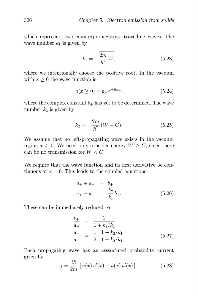
We require that the wave function and its first derivative be continuous at x = 0. This leads to the coupled equations
a + + a − = b +
k 2
a + − a − =
b + .
(5.26)
k 1
These can be immediately reduced to
b +
2
=
a +
1 + k 2 /k 1
a −
1 1 − k 2 /k 1
=
·
.
(5.27)
a +
2 1 + k 2 /k 1
Each propagating wave has an asssociated probability current
given by
j =
i¯ h
2m
[ u(x) ¯
u
� (x) − ¯
u(x) u
� (x) ] .
(5.28)
306
Chapter 5. Electron emission from solids
wave number k 1 is given by
2m
k 1 =
W ,
(5.23)
h
2
¯
where we intentionally choose the positive root. In the vacuum
with x ≥ 0 the wave function is
+ik 2 x
u(x ≥ 0) = b + e
,
(5.24)
where the complex constant b + has yet to be determined. The wave
number k 2 is given by
2m
k 2 =
(W − C),
(5.25)
h
2
¯
We assume that no left-propagating wave exists in the vacuum
region x ≥ 0. We need only consider energy W ≥ C, since there
can be no transmission for W < C.
We require that the wave function and its first derivative be continuous at x = 0. This leads to the coupled equations
a + + a − = b +
k 2
a + − a − =
b + .
(5.26)
k 1
These can be immediately reduced to
b +
2
=
a +
1 + k 2 /k 1
a −
1 1 − k 2 /k 1
=
·
.
(5.27)
a +
2 1 + k 2 /k 1
Each propagating wave has an asssociated probability current
given by
j =
i¯ h
2m
[ u(x) ¯
u
� (x) − ¯
u(x) u
� (x) ] .
(5.28)
306
Chapter 5. Electron emission from solids