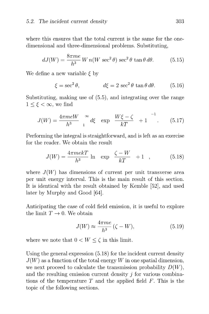
�
�
�
�
where this ensures that the total current is the same for the onedimensional and three-dimensional problems. Substituting,
dJ(W ) =
8πme W n(W sec
2 θ) sec
2 θ tan θ dθ.
(5.15)
h 3
We define a new variable ξ by
ξ = sec
2 θ,
dξ = 2 sec
2 θ tan θ dθ.
(5.16)
Substituting, making use of (5.5), and integrating over the range
1 ≤ ξ < ∞, we find
4πmeW ∞
W ξ − ζ
−1
J(W ) =
dξ exp
+ 1
.
(5.17)
h 3
1
kT
Performing the integral is straightforward, and is left as an exercise
for the reader. We obtain the result
4πmekT
ζ − W
J(W ) =
h 3
ln exp
kT
+ 1 ,
(5.18)
where J(W ) has dimensions of current per unit transverse area
per unit energy interval. This is the main result of this section.
It is identical with the result obtained by Kemble [52], and used
later by Murphy and Good [64].
Anticipating the case of cold field emission, it is useful to explore
the limit T → 0. We obtain
4πme
J(W ) ≈
(ζ − W ),
(5.19)
h 3
where we note that 0 < W ≤ ζ in this limit.
Using the general expression (5.18) for the incident current density
J(W ) as a function of the total energy W in one spatial dimension,
we next proceed to calculate the transmission probability D(W ),
and the resulting emission current density j for various combinations of the temperature T and the applied field F . This is the
topic of the following sections.
303
5.2. The incident current density