

�
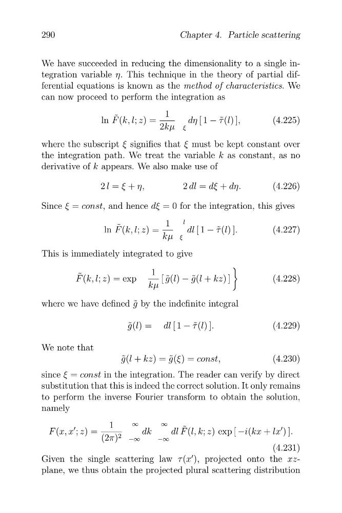
We have succeeded in reducing the dimensionality to a single integration variable η. This technique in the theory of partial differential equations is known as the method of characteristics. We
can now proceed to perform the integration as
1
˜
ln F (k, l; z) =
dη [ 1 − τ ˜(l) ],
(4.225)
2kµ ξ
where the subscript ξ signifies that ξ must be kept constant over
the integration path. We treat the variable k as constant, as no
derivative of k appears. We also make use of
2 l = ξ + η,
2 dl = dξ + dη.
(4.226)
Since ξ = const, and hence dξ = 0 for the integration, this gives
l
1
˜
ln F (k, l; z) =
dl [ 1 − τ ˜(l) ].
(4.227)
kµ ξ
This is immediately integrated to give
1
˜
F (k, l; z) = exp
[ ˜
g(l) − g ˜(l + kz) ]
(4.228)
kµ
where we have defined ˜
g by the indefinite integral
g ˜(l) = dl [ 1 − τ ˜(l) ].
(4.229)
We note that
g ˜(l + kz) = ˜
g(ξ) = const,
(4.230)
since ξ = const in the integration. The reader can verify by direct
substitution that this is indeed the correct solution. It only remains
to perform the inverse Fourier transform to obtain the solution,
namely
F (x, x
� ; z) =
1
∞
dk
∞
dl F ˜ (l, k; z) exp [ −i(kx + lx
� ) ].
(2π) 2 −∞
−∞
(4.231)
Given the single scattering law τ (x
� ), projected onto the xzplane, we thus obtain the projected plural scattering distribution
290
Chapter 4. Particle scattering
We have succeeded in reducing the dimensionality to a single integration variable η. This technique in the theory of partial differential equations is known as the method of characteristics. We
can now proceed to perform the integration as
1
˜
ln F (k, l; z) =
dη [ 1 − τ ˜(l) ],
(4.225)
2kµ ξ
where the subscript ξ signifies that ξ must be kept constant over
the integration path. We treat the variable k as constant, as no
derivative of k appears. We also make use of
2 l = ξ + η,
2 dl = dξ + dη.
(4.226)
Since ξ = const, and hence dξ = 0 for the integration, this gives
l
1
˜
ln F (k, l; z) =
dl [ 1 − τ ˜(l) ].
(4.227)
kµ ξ
This is immediately integrated to give
1
˜
F (k, l; z) = exp
[ ˜
g(l) − g ˜(l + kz) ]
(4.228)
kµ
where we have defined ˜
g by the indefinite integral
g ˜(l) = dl [ 1 − τ ˜(l) ].
(4.229)
We note that
g ˜(l + kz) = ˜
g(ξ) = const,
(4.230)
since ξ = const in the integration. The reader can verify by direct
substitution that this is indeed the correct solution. It only remains
to perform the inverse Fourier transform to obtain the solution,
namely
F (x, x
� ; z) =
1
∞
dk
∞
dl F ˜ (l, k; z) exp [ −i(kx + lx
� ) ].
(2π) 2 −∞
−∞
(4.231)
Given the single scattering law τ (x
� ), projected onto the xzplane, we thus obtain the projected plural scattering distribution
290
Chapter 4. Particle scattering