

250
Chapter 4. Particle scattering
This applies to any case with axial symmetry, regardless of the
detailed dependence of the scattering force on the separation r.
We assume that all relevant information about the scattering
forces is contained in the potential energy U (x) between the two
particles, where x is the three-vector spatial separation between
the particles. We assume U to be known. For the present analysis
we now consider the special case for which the potential energy
can be written as
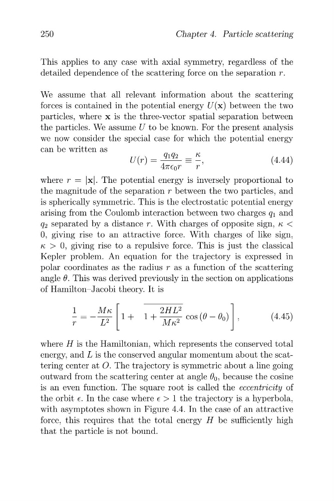
q 1 q 2
κ
U (r) =
≡ ,
(4.44)
4πf 0 r
r
where r = |x|. The potential energy is inversely proportional to
the magnitude of the separation r between the two particles, and
is spherically symmetric. This is the electrostatic potential energy
arising from the Coulomb interaction between two charges q 1 and
q 2 separated by a distance r. With charges of opposite sign, κ <
0, giving rise to an attractive force. With charges of like sign,
κ > 0, giving rise to a repulsive force. This is just the classical
Kepler problem. An equation for the trajectory is expressed in
polar coordinates as the radius r as a function of the scattering
angle θ. This was derived previously in the section on applications
of Hamilton–Jacobi theory. It is
⎡
⎤
1
M κ
2HL 2
= −
⎣ 1 + 1 +
cos (θ − θ 0 ) ⎦ ,
(4.45)
r
L 2
M κ 2
where H is the Hamiltonian, which represents the conserved total
energy, and L is the conserved angular momentum about the scattering center at O. The trajectory is symmetric about a line going
outward from the scattering center at angle θ 0 , because the cosine
is an even function. The square root is called the eccentricity of
the orbit f. In the case where f > 1 the trajectory is a hyperbola,
with asymptotes shown in Figure 4.4. In the case of an attractive
force, this requires that the total energy H be sufficiently high
that the particle is not bound.
Chapter 4. Particle scattering
This applies to any case with axial symmetry, regardless of the
detailed dependence of the scattering force on the separation r.
We assume that all relevant information about the scattering
forces is contained in the potential energy U (x) between the two
particles, where x is the three-vector spatial separation between
the particles. We assume U to be known. For the present analysis
we now consider the special case for which the potential energy
can be written as
q 1 q 2
κ
U (r) =
≡ ,
(4.44)
4πf 0 r
r
where r = |x|. The potential energy is inversely proportional to
the magnitude of the separation r between the two particles, and
is spherically symmetric. This is the electrostatic potential energy
arising from the Coulomb interaction between two charges q 1 and
q 2 separated by a distance r. With charges of opposite sign, κ <
0, giving rise to an attractive force. With charges of like sign,
κ > 0, giving rise to a repulsive force. This is just the classical
Kepler problem. An equation for the trajectory is expressed in
polar coordinates as the radius r as a function of the scattering
angle θ. This was derived previously in the section on applications
of Hamilton–Jacobi theory. It is
⎡
⎤
1
M κ
2HL 2
= −
⎣ 1 + 1 +
cos (θ − θ 0 ) ⎦ ,
(4.45)
r
L 2
M κ 2
where H is the Hamiltonian, which represents the conserved total
energy, and L is the conserved angular momentum about the scattering center at O. The trajectory is symmetric about a line going
outward from the scattering center at angle θ 0 , because the cosine
is an even function. The square root is called the eccentricity of
the orbit f. In the case where f > 1 the trajectory is a hyperbola,
with asymptotes shown in Figure 4.4. In the case of an attractive
force, this requires that the total energy H be sufficiently high
that the particle is not bound.