

�
�
�
�
3.2. Particle motion in a general electromagnetic potential 183
which we immediately recognize from the relationship (2.25) between the canonical momentum P and the kinetic momentum p.
We have neglected the negative root. This means that we only
consider motion in the forward direction for the present purpose.
Integrating, we obtain
x b
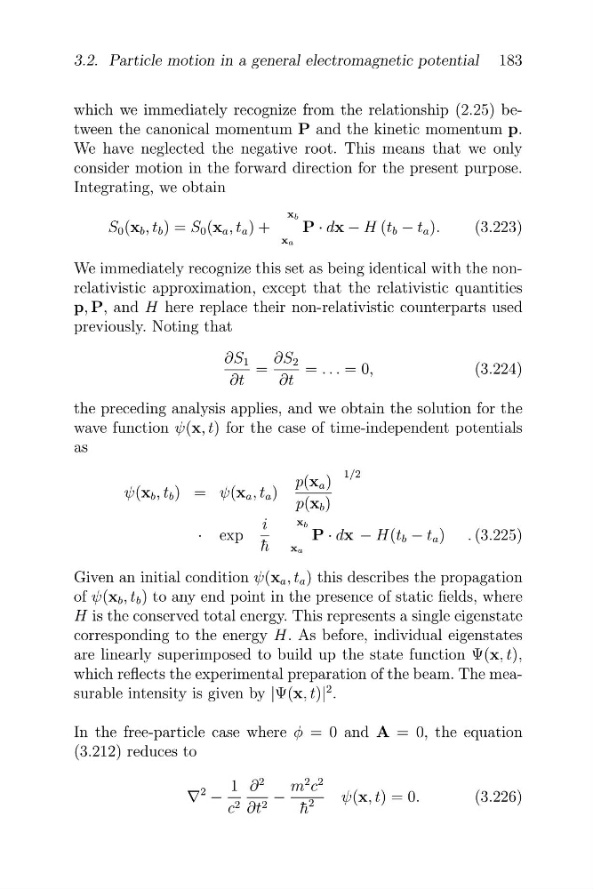
S 0 (x b , t b ) = S 0 (x a , t a ) +
P · dx − H (t b − t a ).
(3.223)
xa
We immediately recognize this set as being identical with the nonrelativistic approximation, except that the relativistic quantities
p, P, and H here replace their non-relativistic counterparts used
previously. Noting that
∂S 1
∂S 2
=
= . . . = 0,
(3.224)
∂t
∂t
the preceding analysis applies, and we obtain the solution for the
wave function ψ(x, t) for the case of time-independent potentials
as
1/2
p(x a )
ψ(x b , t b ) = ψ(x a , t a ) p(x b )
i
x b
· exp
P · dx − H(t b − t a ) . (3.225)
h ¯ xa
Given an initial condition ψ(x a , t a ) this describes the propagation
of ψ(x b , t b ) to any end point in the presence of static fields, where
H is the conserved total energy. This represents a single eigenstate
corresponding to the energy H. As before, individual eigenstates
are linearly superimposed to build up the state function Ψ(x, t),
which reflects the experimental preparation of the beam. The measurable intensity is given by |Ψ(x, t)|
2 .
In the free-particle case where φ = 0 and A = 0, the equation
(3.212) reduces to
1 ∂
2
m
2 c
2
v
2 −
−
ψ(x, t) = 0.
(3.226)
c 2 ∂t 2
h ¯
2
�
�
�
3.2. Particle motion in a general electromagnetic potential 183
which we immediately recognize from the relationship (2.25) between the canonical momentum P and the kinetic momentum p.
We have neglected the negative root. This means that we only
consider motion in the forward direction for the present purpose.
Integrating, we obtain
x b
S 0 (x b , t b ) = S 0 (x a , t a ) +
P · dx − H (t b − t a ).
(3.223)
xa
We immediately recognize this set as being identical with the nonrelativistic approximation, except that the relativistic quantities
p, P, and H here replace their non-relativistic counterparts used
previously. Noting that
∂S 1
∂S 2
=
= . . . = 0,
(3.224)
∂t
∂t
the preceding analysis applies, and we obtain the solution for the
wave function ψ(x, t) for the case of time-independent potentials
as
1/2
p(x a )
ψ(x b , t b ) = ψ(x a , t a ) p(x b )
i
x b
· exp
P · dx − H(t b − t a ) . (3.225)
h ¯ xa
Given an initial condition ψ(x a , t a ) this describes the propagation
of ψ(x b , t b ) to any end point in the presence of static fields, where
H is the conserved total energy. This represents a single eigenstate
corresponding to the energy H. As before, individual eigenstates
are linearly superimposed to build up the state function Ψ(x, t),
which reflects the experimental preparation of the beam. The measurable intensity is given by |Ψ(x, t)|
2 .
In the free-particle case where φ = 0 and A = 0, the equation
(3.212) reduces to
1 ∂
2
m
2 c
2
v
2 −
−
ψ(x, t) = 0.
(3.226)
c 2 ∂t 2
h ¯
2