

136
Chapter 3. Wave optics
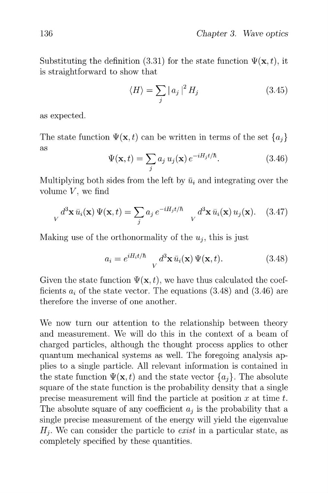
Substituting the definition (3.31) for the state function Ψ(x, t), it
is straightforward to show that
4
(H) =
| a j |
2 H j
(3.45)
j
as expected.
The state function Ψ(x, t) can be written in terms of the set {a j }
as
4
−iH j t/¯ h
Ψ(x, t) =
a j u j (x) e
.
(3.46)
j
Multiplying both sides from the left by ¯
u i and integrating over the
volume V , we find
4
−iH j t/¯ h
d
3
d
3
x u ¯ i (x) Ψ(x, t) =
a j e
x u ¯ i (x) u j (x). (3.47)
V
V
j
Making use of the orthonormality of the u j , this is just
iH i t/¯ h
d
3
a i = e
x u ¯ i (x) Ψ(x, t).
(3.48)
V
Given the state function Ψ(x, t), we have thus calculated the coefficients a i of the state vector. The equations (3.48) and (3.46) are
therefore the inverse of one another.
We now turn our attention to the relationship between theory
and measurement. We will do this in the context of a beam of
charged particles, although the thought process applies to other
quantum mechanical systems as well. The foregoing analysis applies to a single particle. All relevant information is contained in
the state function Ψ(x, t) and the state vector {a j }. The absolute
square of the state function is the probability density that a single
precise measurement will find the particle at position x at time t.
The absolute square of any coefficient a j is the probability that a
single precise measurement of the energy will yield the eigenvalue
H j . We can consider the particle to exist in a particular state, as
completely specified by these quantities.
Chapter 3. Wave optics
Substituting the definition (3.31) for the state function Ψ(x, t), it
is straightforward to show that
4
(H) =
| a j |
2 H j
(3.45)
j
as expected.
The state function Ψ(x, t) can be written in terms of the set {a j }
as
4
−iH j t/¯ h
Ψ(x, t) =
a j u j (x) e
.
(3.46)
j
Multiplying both sides from the left by ¯
u i and integrating over the
volume V , we find
4
−iH j t/¯ h
d
3
d
3
x u ¯ i (x) Ψ(x, t) =
a j e
x u ¯ i (x) u j (x). (3.47)
V
V
j
Making use of the orthonormality of the u j , this is just
iH i t/¯ h
d
3
a i = e
x u ¯ i (x) Ψ(x, t).
(3.48)
V
Given the state function Ψ(x, t), we have thus calculated the coefficients a i of the state vector. The equations (3.48) and (3.46) are
therefore the inverse of one another.
We now turn our attention to the relationship between theory
and measurement. We will do this in the context of a beam of
charged particles, although the thought process applies to other
quantum mechanical systems as well. The foregoing analysis applies to a single particle. All relevant information is contained in
the state function Ψ(x, t) and the state vector {a j }. The absolute
square of the state function is the probability density that a single
precise measurement will find the particle at position x at time t.
The absolute square of any coefficient a j is the probability that a
single precise measurement of the energy will yield the eigenvalue
H j . We can consider the particle to exist in a particular state, as
completely specified by these quantities.