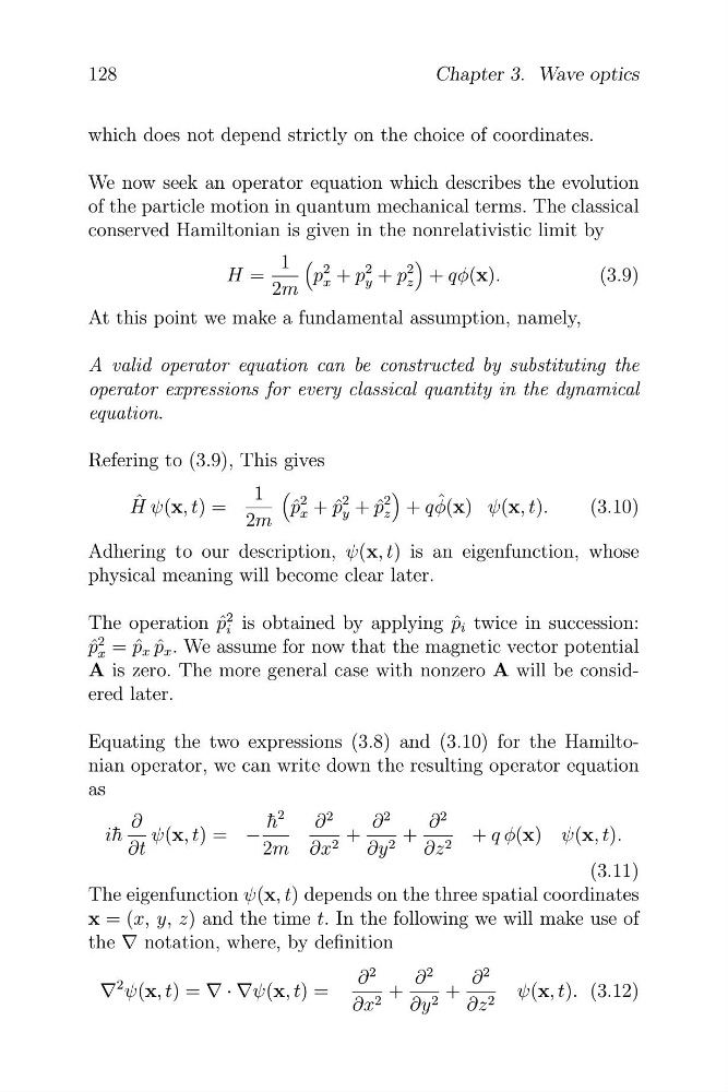
�
�
�
�
�
�
which does not depend strictly on the choice of coordinates.
We now seek an operator equation which describes the evolution
of the particle motion in quantum mechanical terms. The classical
conserved Hamiltonian is given in the nonrelativistic limit by
1
2
2
2
H =
p + p + p + qφ(x).
(3.9)
x
y
z
2m
At this point we make a fundamental assumption, namely,
A valid operator equation can be constructed by substituting the
operator expressions for every classical quantity in the dynamical
equation.
Refering to (3.9), This gives
1
2
2
2
ˆ
ˆ
H ψ(x, t) =
p ˆ x + ˆ
p y + ˆ
p z + qφ(x) ψ(x, t).
(3.10)
2m
Adhering to our description, ψ(x, t) is an eigenfunction, whose
physical meaning will become clear later.
The operation ˆ
p
2
i is obtained by applying ˆ
p i twice in succession:
p ˆ
2 = ˆ p ˆ x . We assume for now that the magnetic vector potential
x
p x
A is zero. The more general case with nonzero A will be considered later.
Equating the two expressions (3.8) and (3.10) for the Hamiltonian operator, we can write down the resulting operator equation
as
∂
h ¯
2
∂
2
∂
2
∂
2
ih ¯
ψ(x, t) = −
+
+
+ q φ(x) ψ(x, t).
∂t
2m ∂x 2 ∂y 2 ∂z 2
(3.11)
The eigenfunction ψ(x, t) depends on the three spatial coordinates
x = (x, y, z) and the time t. In the following we will make use of
the v notation, where, by definition
∂
2
∂
2
∂
2
v
2 ψ(x, t) = v · vψ(x, t) =
+
+
ψ(x, t). (3.12)
∂x 2 ∂y 2 ∂z 2
128
Chapter 3. Wave optics