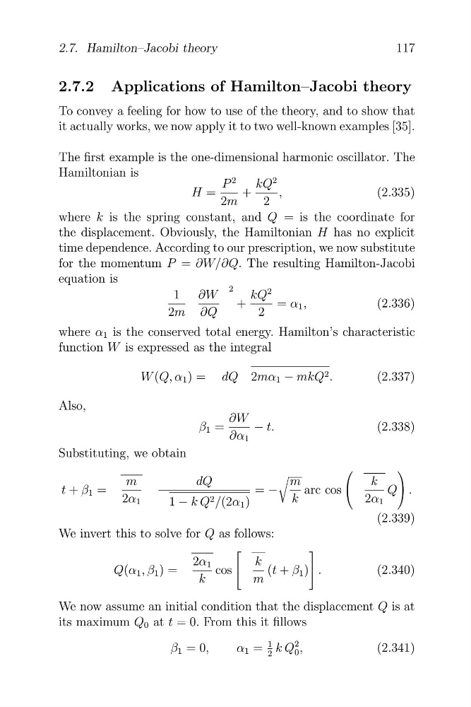
�
�
�
The first example is the one-dimensional harmonic oscillator. The
Hamiltonian is
P
2
kQ
2
H =
+
,
(2.335)
2m
2
where k is the spring constant, and Q = is the coordinate for
the displacement. Obviously, the Hamiltonian H has no explicit
time dependence. According to our prescription, we now substitute
for the momentum P = ∂W/∂Q. The resulting Hamilton-Jacobi
equation is
1 ∂W
2
kQ
2
+
= α 1 ,
(2.336)
2m ∂Q
2
where α 1 is the conserved total energy. Hamilton’s characteristic
function W is expressed as the integral
W (Q, α 1 ) = dQ 2mα 1 − mkQ 2 .
(2.337)
Also,
∂W
β 1 =
− t.
(2.338)
∂α 1
Substituting, we obtain
⎛
⎞
m
dQ
m
k
t + β 1 =
= −
arc cos ⎝
Q ⎠ .
2α 1
1 − k Q 2 /(2α 1 )
k
2α 1
(2.339)
We invert this to solve for Q as follows:
⎡
⎤
2α 1
k
Q(α 1 , β 1 ) =
cos ⎣
(t + β 1 ) ⎦ .
(2.340)
k
m
We now assume an initial condition that the displacement Q is at
its maximum Q 0 at t = 0. From this it fillows
β 1 = 0,
=
1 k Q
2
(2.341)
α 1 2
0 ,
117
2.7. Hamilton–Jacobi theory
2.7.2 Applications of Hamilton–Jacobi theory
To convey a feeling for how to use of the theory, and to show that
it actually works, we now apply it to two well-known examples [35].