

�
�
112
Chapter 2. Geometrical optics
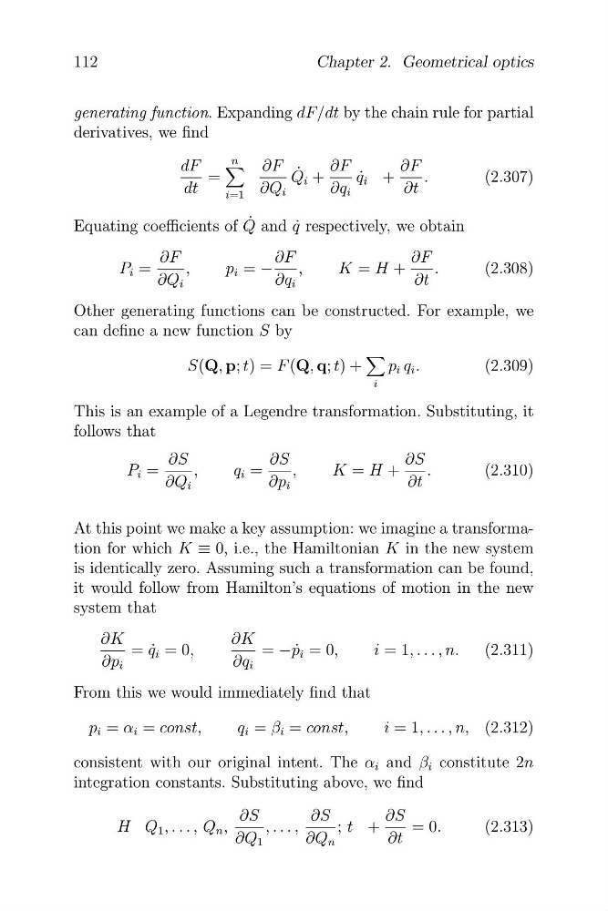
generating function. Expanding dF/dt by the chain rule for partial
derivatives, we find
4
dF
n
∂F
∂F
∂F
˙
=
Q i +
q˙ i +
.
(2.307)
dt
i=1 ∂Q i
∂q i
∂t
˙
Equating coefficients of Q and ˙
q respectively, we obtain
∂F
∂F
∂F
P i =
,
p i = −
,
K = H +
.
(2.308)
∂Q i
∂q i
∂t
Other generating functions can be constructed. For example, we
can define a new function S by
4
S(Q, p; t) = F (Q, q; t) +
p i q i .
(2.309)
i
This is an example of a Legendre transformation. Substituting, it
follows that
∂S
∂S
∂S
P i =
,
q i =
,
K = H +
.
(2.310)
∂Q i
∂p i
∂t
At this point we make a key assumption: we imagine a transformation for which K ≡ 0, i.e., the Hamiltonian K in the new system
is identically zero. Assuming such a transformation can be found,
it would follow from Hamilton’s equations of motion in the new
system that
∂K
∂K
= q˙ i = 0,
= −p ˙ i = 0,
i = 1, . . . , n.
(2.311)
∂p i
∂q i
From this we would immediately find that
p i = α i = const,
q i = β i = const,
i = 1, . . . , n, (2.312)
consistent with our original intent. The α i and β i constitute 2n
integration constants. Substituting above, we find
∂S
∂S
∂S
H Q 1 , . . . , Q n ,
, . . . ,
; t +
= 0.
(2.313)
∂Q 1
∂Q n
∂t
�
112
Chapter 2. Geometrical optics
generating function. Expanding dF/dt by the chain rule for partial
derivatives, we find
4
dF
n
∂F
∂F
∂F
˙
=
Q i +
q˙ i +
.
(2.307)
dt
i=1 ∂Q i
∂q i
∂t
˙
Equating coefficients of Q and ˙
q respectively, we obtain
∂F
∂F
∂F
P i =
,
p i = −
,
K = H +
.
(2.308)
∂Q i
∂q i
∂t
Other generating functions can be constructed. For example, we
can define a new function S by
4
S(Q, p; t) = F (Q, q; t) +
p i q i .
(2.309)
i
This is an example of a Legendre transformation. Substituting, it
follows that
∂S
∂S
∂S
P i =
,
q i =
,
K = H +
.
(2.310)
∂Q i
∂p i
∂t
At this point we make a key assumption: we imagine a transformation for which K ≡ 0, i.e., the Hamiltonian K in the new system
is identically zero. Assuming such a transformation can be found,
it would follow from Hamilton’s equations of motion in the new
system that
∂K
∂K
= q˙ i = 0,
= −p ˙ i = 0,
i = 1, . . . , n.
(2.311)
∂p i
∂q i
From this we would immediately find that
p i = α i = const,
q i = β i = const,
i = 1, . . . , n, (2.312)
consistent with our original intent. The α i and β i constitute 2n
integration constants. Substituting above, we find
∂S
∂S
∂S
H Q 1 , . . . , Q n ,
, . . . ,
; t +
= 0.
(2.313)
∂Q 1
∂Q n
∂t