

�
�
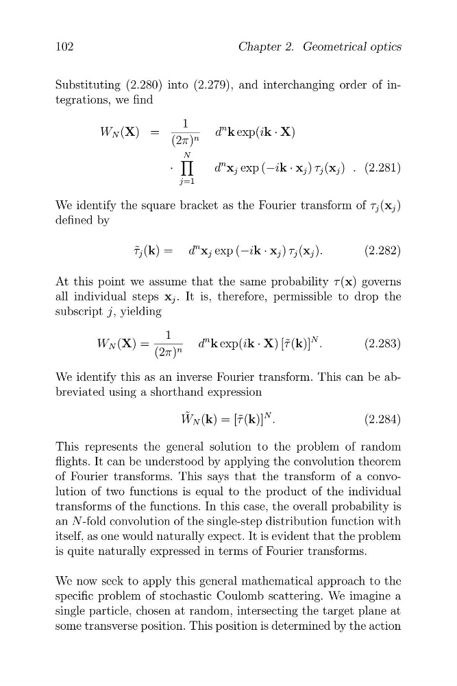
Substituting (2.280) into (2.279), and interchanging order of integrations, we find
1
W N (X) = (2π) n d
n k exp(ik · X)
N
N
·
d
n x j exp (−ik · x j ) τ j (x j ) . (2.281)
j=1
We identify the square bracket as the Fourier transform of τ j (x j )
defined by
τ ˜ j (k) = d
n x j exp (−ik · x j ) τ j (x j ).
(2.282)
At this point we assume that the same probability τ (x) governs
all individual steps x j . It is, therefore, permissible to drop the
subscript j, yielding
W N (X) =
1
d
n k exp(ik · X) [˜ τ (k)]
N .
(2.283)
(2π) n
We identify this as an inverse Fourier transform. This can be abbreviated using a shorthand expression
W ˜ N (k) = [˜ τ (k)]
N .
(2.284)
102
Chapter 2. Geometrical optics
This represents the general solution to the problem of random
flights. It can be understood by applying the convolution theorem
of Fourier transforms. This says that the transform of a convolution of two functions is equal to the product of the individual
transforms of the functions. In this case, the overall probability is
an N -fold convolution of the single-step distribution function with
itself, as one would naturally expect. It is evident that the problem
is quite naturally expressed in terms of Fourier transforms.
We now seek to apply this general mathematical approach to the
specific problem of stochastic Coulomb scattering. We imagine a
single particle, chosen at random, intersecting the target plane at
some transverse position. This position is determined by the action
�
Substituting (2.280) into (2.279), and interchanging order of integrations, we find
1
W N (X) = (2π) n d
n k exp(ik · X)
N
N
·
d
n x j exp (−ik · x j ) τ j (x j ) . (2.281)
j=1
We identify the square bracket as the Fourier transform of τ j (x j )
defined by
τ ˜ j (k) = d
n x j exp (−ik · x j ) τ j (x j ).
(2.282)
At this point we assume that the same probability τ (x) governs
all individual steps x j . It is, therefore, permissible to drop the
subscript j, yielding
W N (X) =
1
d
n k exp(ik · X) [˜ τ (k)]
N .
(2.283)
(2π) n
We identify this as an inverse Fourier transform. This can be abbreviated using a shorthand expression
W ˜ N (k) = [˜ τ (k)]
N .
(2.284)
102
Chapter 2. Geometrical optics
This represents the general solution to the problem of random
flights. It can be understood by applying the convolution theorem
of Fourier transforms. This says that the transform of a convolution of two functions is equal to the product of the individual
transforms of the functions. In this case, the overall probability is
an N -fold convolution of the single-step distribution function with
itself, as one would naturally expect. It is evident that the problem
is quite naturally expressed in terms of Fourier transforms.
We now seek to apply this general mathematical approach to the
specific problem of stochastic Coulomb scattering. We imagine a
single particle, chosen at random, intersecting the target plane at
some transverse position. This position is determined by the action