

N
4
W N (X) = · · · δ ⎝
x j − X ⎠ τ 1 (x 1 ) · · · τ N (x N ) · dx 1 · · · dx N ,
j=1
(2.279)
where δ is the Dirac delta function, which ensures that only that
space is included in the integration, for which the constraint is
met. The delta function has an integral representation given by
⎛
⎞
⎡
⎛
⎞⎤
N
N
4
4
1
⎠
δ ⎝
x j − X ⎠ =
d
n k exp ⎣ −ik · ⎝
x j − X ⎦ ,
(2π) n
j=1
j=1
(2.280)
where the integral is performed over the entire n-dimensional space
of the n-vector k.
⎛
⎞
101
2.6. Stochastic Coulomb scattering
ulation. To this end, we first discuss of the problem of random
flights, originally formulated and solved by Markov, and reviewed
by Chandrasekhar [17]. We imagine a general physical process consisting of a number of independent steps of varying size. For example, the process might be the motion of a gas molecule, where
the molecule is multiply scattered. Between scattering events, the
molecule travels a random distance, which represents the length
of a step. We wish to determine the probability that the molecule
travels a given net distance after N scattering events. There are
many other examples of this general process. A key assumption is
that the probability of a single event is independent of past history. Such a succession of events is known as a Markov chain.
In mathematical terms, the problem can be stated as follows. We
assume the size of the jth step is governed by a probability density τ j (x j ) that the step length will be x j . Given this, we wish to
find the probability density W N (X) for net displacement X after
N steps with displacements x j , where j = 1, . . . , N . This is completely general, in that the vector quantities x and X can have
any dimensionality. The probability W N (X) is found by integrating over all possible step lengths x j , subject to the constraint that
the individual steps must add up to give the desired displacement
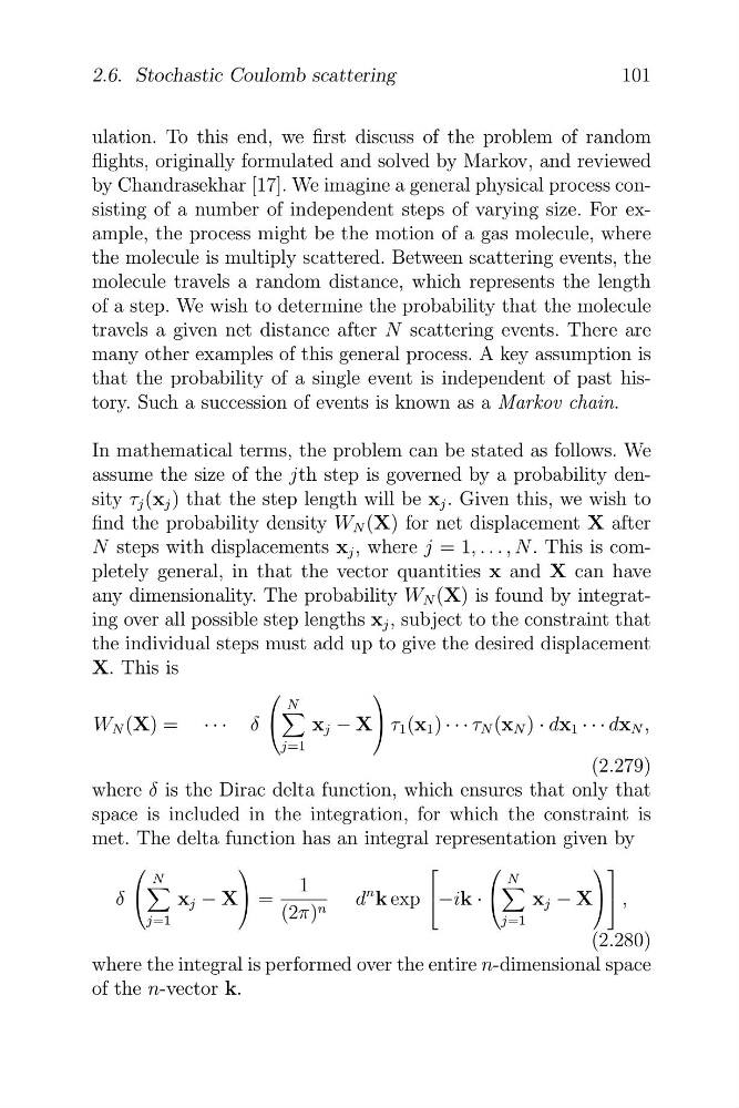
X. This is
4
W N (X) = · · · δ ⎝
x j − X ⎠ τ 1 (x 1 ) · · · τ N (x N ) · dx 1 · · · dx N ,
j=1
(2.279)
where δ is the Dirac delta function, which ensures that only that
space is included in the integration, for which the constraint is
met. The delta function has an integral representation given by
⎛
⎞
⎡
⎛
⎞⎤
N
N
4
4
1
⎠
δ ⎝
x j − X ⎠ =
d
n k exp ⎣ −ik · ⎝
x j − X ⎦ ,
(2π) n
j=1
j=1
(2.280)
where the integral is performed over the entire n-dimensional space
of the n-vector k.
⎛
⎞
101
2.6. Stochastic Coulomb scattering
ulation. To this end, we first discuss of the problem of random
flights, originally formulated and solved by Markov, and reviewed
by Chandrasekhar [17]. We imagine a general physical process consisting of a number of independent steps of varying size. For example, the process might be the motion of a gas molecule, where
the molecule is multiply scattered. Between scattering events, the
molecule travels a random distance, which represents the length
of a step. We wish to determine the probability that the molecule
travels a given net distance after N scattering events. There are
many other examples of this general process. A key assumption is
that the probability of a single event is independent of past history. Such a succession of events is known as a Markov chain.
In mathematical terms, the problem can be stated as follows. We
assume the size of the jth step is governed by a probability density τ j (x j ) that the step length will be x j . Given this, we wish to
find the probability density W N (X) for net displacement X after
N steps with displacements x j , where j = 1, . . . , N . This is completely general, in that the vector quantities x and X can have
any dimensionality. The probability W N (X) is found by integrating over all possible step lengths x j , subject to the constraint that
the individual steps must add up to give the desired displacement
X. This is