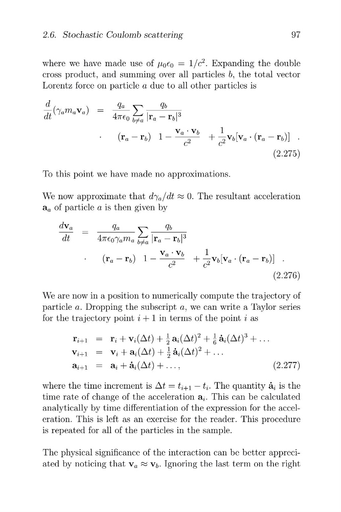
where we have made use of µ 0 f 0 = 1/c
2 . Expanding the double
cross product, and summing over all particles b, the total vector
Lorentz force on particle a due to all other particles is
4
d
q a
q b
(γ a m a v a ) =
dt
4πf 0
|r a − r b | 3
b=a
v a · v b
1
·
(r a − r b ) 1 −
2
+ 2 v b [v a · (r a − r b )] .
c
c
(2.275)
To this point we have made no approximations.
We now approximate that dγ a /dt ≈ 0. The resultant acceleration
a a of particle a is then given by
4
dv a
q a
q b
=
dt
4πf 0 γ a m a
|r a − r b | 3
b=a
·
(r a − r b ) 1 −
v a · v b
c 2
+
1
c 2 v b [v a · (r a − r b )] .
(2.276)
We are now in a position to numerically compute the trajectory of
particle a. Dropping the subscript a, we can write a Taylor series
for the trajectory point i + 1 in terms of the point i as
r i+1 = r i + v i (Δt) +
1
2
a i (Δt)
2 +
1
6
a ˙ i (Δt)
3 + . . .

v i+1 = v i + a i (Δt) +
1
2
a ˙ i (Δt)
2 + . . .

a i+1 = a i + a ˙ i (Δt) + . . . ,
(2.277)

where the time increment is Δt = t i+1 − t i . The quantity a ˙ i is the
time rate of change of the acceleration a i . This can be calculated
analytically by time differentiation of the expression for the acceleration. This is left as an exercise for the reader. This procedure
is repeated for all of the particles in the sample.
The physical significance of the interaction can be better appreciated by noticing that v a ≈ v b . Ignoring the last term on the right
97
2.6. Stochastic Coulomb scattering
�
�