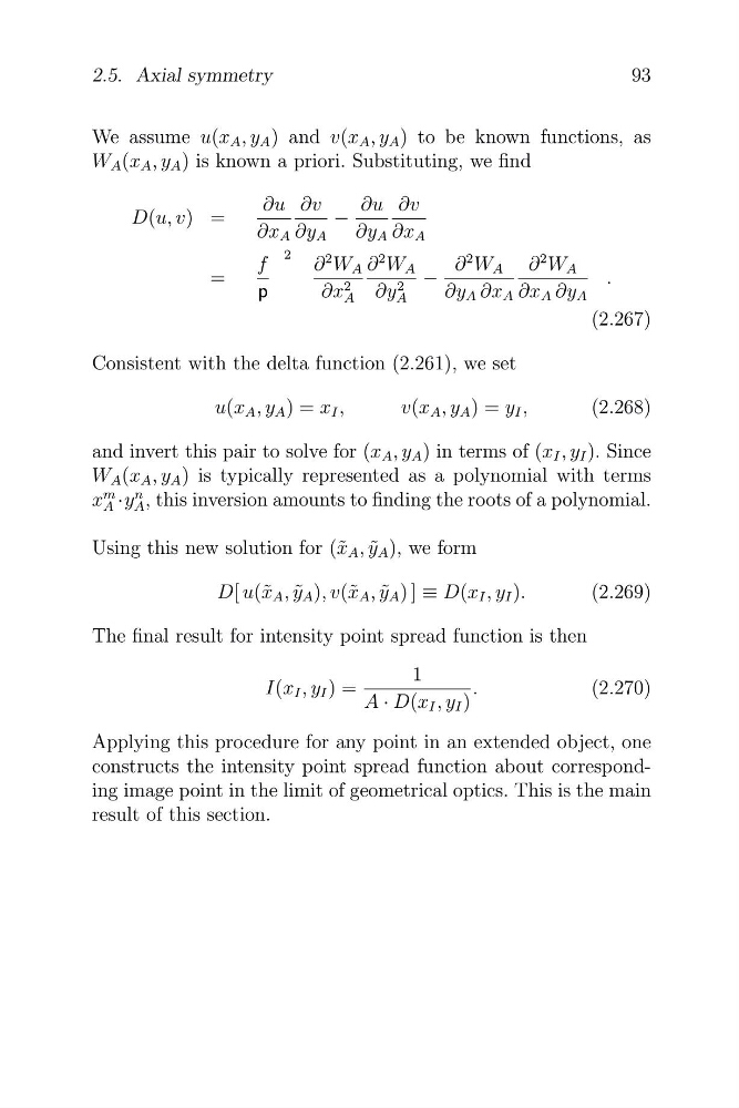
�
�
� � �
�
We assume u(x A , y A ) and v(x A , y A ) to be known functions, as
W A (x A , y A ) is known a priori. Substituting, we find
∂u ∂v
∂u ∂v
D(u, v) =
−
∂x A ∂y A ∂y A ∂x A
f
2
∂
2 W A ∂
2 W A
∂
2 W A ∂
2 W A
=
−
.
p
∂x
2
∂y A
2
∂y A ∂x A
A
∂x A ∂y A
(2.267)
Consistent with the delta function (2.261), we set
u(x A , y A ) = x I ,
v(x A , y A ) = y I ,
(2.268)
and invert this pair to solve for (x A , y A ) in terms of (x I , y I ). Since
W A (x A , y A ) is typically represented as a polynomial with terms
m n
x A ·y A , this inversion amounts to finding the roots of a polynomial.
Using this new solution for (˜ x A , y ˜ A ), we form
D[ u(˜ x A , y ˜ A ), v(˜ x A , y ˜ A ) ] ≡ D(x I , y I ).
(2.269)
The final result for intensity point spread function is then
1
I(x I , y I ) =
.
(2.270)
A · D(x I , y I )
Applying this procedure for any point in an extended object, one
constructs the intensity point spread function about corresponding image point in the limit of geometrical optics. This is the main
result of this section.
93
2.5. Axial symmetry