

(δv 1 )
�� + p
−2 Φ
� (1 + Φ) (δv 1 )
�
1
−2 B
2
+ 2 p
−2 Φ
�� (1 + Φ) + 4
1 p
(δv 1 )
= (δΦ) p
−2 { (2 p
−2 + 1) Φ
� v
�
+
1 [ (2 p
−2 + 1) Φ
�� + p
−2 (1 + Φ) B
2 ] v }, (2.241)
2
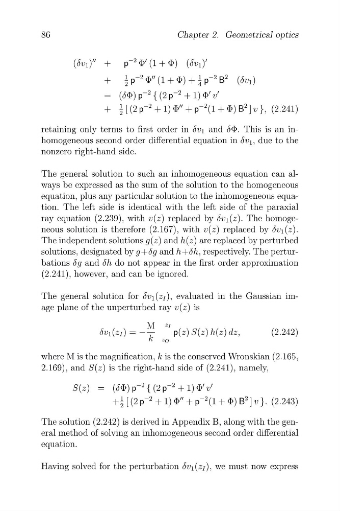
retaining only terms to first order in δv 1 and δΦ. This is an inhomogeneous second order differential equation in δv 1 , due to the
nonzero right-hand side.
The general solution to such an inhomogeneous equation can always be expressed as the sum of the solution to the homogeneous
equation, plus any particular solution to the inhomogeneous equation. The left side is identical with the left side of the paraxial
ray equation (2.239), with v(z) replaced by δv 1 (z). The homogeneous solution is therefore (2.167), with v(z) replaced by δv 1 (z).
The independent solutions g(z) and h(z) are replaced by perturbed
solutions, designated by g+δg and h+δh, respectively. The perturbations δg and δh do not appear in the first order approximation
(2.241), however, and can be ignored.
The general solution for δv 1 (z I ), evaluated in the Gaussian image plane of the unperturbed ray v(z) is
M z I
δv 1 (z I ) = −
p(z) S(z) h(z) dz,
(2.242)
k z O
where M is the magnification, k is the conserved Wronskian (2.165,
2.169), and S(z) is the right-hand side of (2.241), namely,
S(z) = (δΦ) p
−2 { (2 p
−2 + 1) Φ
� v
�
+
1 [ (2 p
−2 + 1) Φ
�� + p
−2 (1 + Φ) B
2 ] v }. (2.243)
2
The solution (2.242) is derived in Appendix B, along with the general method of solving an inhomogeneous second order differential
equation.
Having solved for the perturbation δv 1 (z I ), we must now express
86
Chapter 2. Geometrical optics
�� + p
−2 Φ
� (1 + Φ) (δv 1 )
�
1
−2 B
2
+ 2 p
−2 Φ
�� (1 + Φ) + 4
1 p
(δv 1 )
= (δΦ) p
−2 { (2 p
−2 + 1) Φ
� v
�
+
1 [ (2 p
−2 + 1) Φ
�� + p
−2 (1 + Φ) B
2 ] v }, (2.241)
2
retaining only terms to first order in δv 1 and δΦ. This is an inhomogeneous second order differential equation in δv 1 , due to the
nonzero right-hand side.
The general solution to such an inhomogeneous equation can always be expressed as the sum of the solution to the homogeneous
equation, plus any particular solution to the inhomogeneous equation. The left side is identical with the left side of the paraxial
ray equation (2.239), with v(z) replaced by δv 1 (z). The homogeneous solution is therefore (2.167), with v(z) replaced by δv 1 (z).
The independent solutions g(z) and h(z) are replaced by perturbed
solutions, designated by g+δg and h+δh, respectively. The perturbations δg and δh do not appear in the first order approximation
(2.241), however, and can be ignored.
The general solution for δv 1 (z I ), evaluated in the Gaussian image plane of the unperturbed ray v(z) is
M z I
δv 1 (z I ) = −
p(z) S(z) h(z) dz,
(2.242)
k z O
where M is the magnification, k is the conserved Wronskian (2.165,
2.169), and S(z) is the right-hand side of (2.241), namely,
S(z) = (δΦ) p
−2 { (2 p
−2 + 1) Φ
� v
�
+
1 [ (2 p
−2 + 1) Φ
�� + p
−2 (1 + Φ) B
2 ] v }. (2.243)
2
The solution (2.242) is derived in Appendix B, along with the general method of solving an inhomogeneous second order differential
equation.
Having solved for the perturbation δv 1 (z I ), we must now express
86
Chapter 2. Geometrical optics