

THz Bandpass Filter Design Using Metamaterial-Based Defected 1D …
5
Let us introduce the vector
ψ(z) =
E(z)
B(z)
=
E(z)
−
i
κ 0
∂ E(z)
∂z
(3.8)
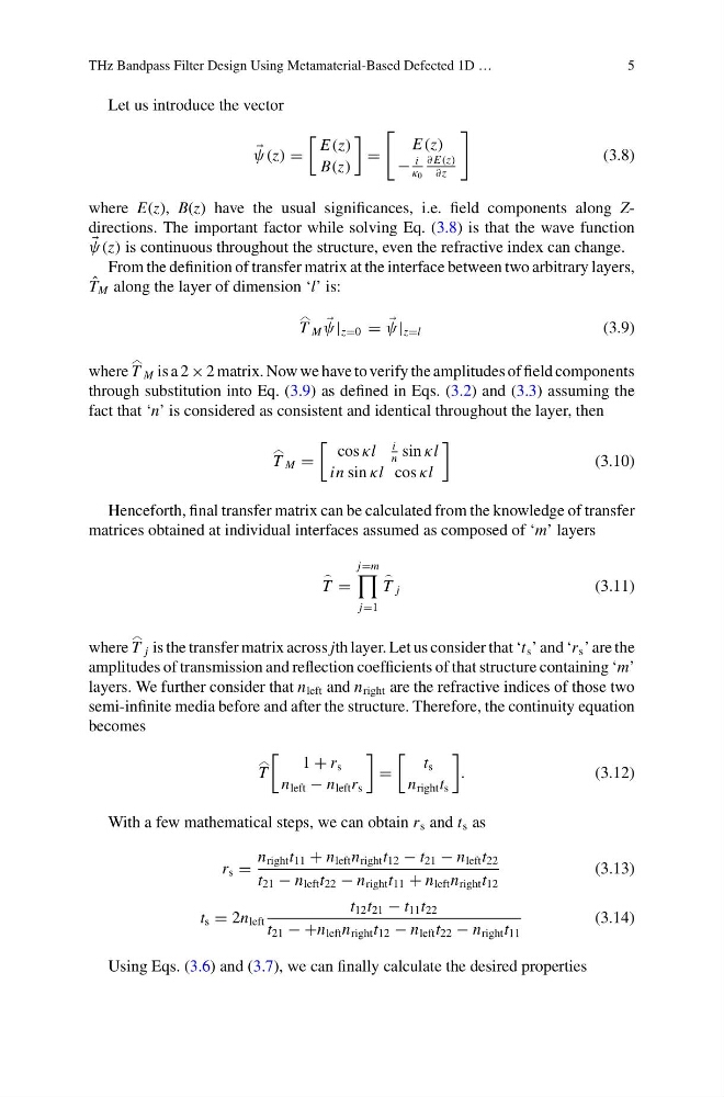
where E(z), B(z) have the usual significances, i.e. field components along Zdirections. The important factor while solving Eq. (3.8) is that the wave function
ψ(z) is continuous throughout the structure, even the refractive index can change.
From the definition of transfer matrix at the interface between two arbitrary layers,
ˆ
T M along the layer of dimension ‘l’ is:
T
M
ψ| z=0 =
ψ| z=l
(3.9)
where T
M is a 2 × 2 matrix. Now we have to verify the amplitudes of field components
through substitution into Eq. (3.9) as defined in Eqs. (3.2) and (3.3) assuming the
fact that ‘n’ is considered as consistent and identical throughout the layer, then
T
M =
cos κl
i
n
sin κl
in sin κl cos κl
(3.10)
Henceforth, final transfer matrix can be calculated from the knowledge of transfer
matrices obtained at individual interfaces assumed as composed of ‘m’ layers
T =
j=m
j=1
T j
(3.11)
where T
j is the transfer matrix across jth layer. Let us consider that ‘t s ’ and ‘r s ’ are the
amplitudes of transmission and reflection coefficients of that structure containing ‘m’
layers. We further consider that n left and n right are the refractive indices of those two
semi-infinite media before and after the structure. Therefore, the continuity equation
becomes
T
1 + r s
n left − n left r s
=
t s
n right t s
.
(3.12)
With a few mathematical steps, we can obtain r s and t s as
r s =
n right t 11 + n left n right t 12 − t 21 − n left t 22
t 21 − n left t 22 − n right t 11 + n left n right t 12
(3.13)
t s = 2n left
t 12 t 21 − t 11 t 22
t 21 − +n left n right t 12 − n left t 22 − n right t 11
(3.14)
Using Eqs. (3.6) and (3.7), we can finally calculate the desired properties
5
Let us introduce the vector
ψ(z) =
E(z)
B(z)
=
E(z)
−
i
κ 0
∂ E(z)
∂z
(3.8)
where E(z), B(z) have the usual significances, i.e. field components along Zdirections. The important factor while solving Eq. (3.8) is that the wave function
ψ(z) is continuous throughout the structure, even the refractive index can change.
From the definition of transfer matrix at the interface between two arbitrary layers,
ˆ
T M along the layer of dimension ‘l’ is:
T
M
ψ| z=0 =
ψ| z=l
(3.9)
where T
M is a 2 × 2 matrix. Now we have to verify the amplitudes of field components
through substitution into Eq. (3.9) as defined in Eqs. (3.2) and (3.3) assuming the
fact that ‘n’ is considered as consistent and identical throughout the layer, then
T
M =
cos κl
i
n
sin κl
in sin κl cos κl
(3.10)
Henceforth, final transfer matrix can be calculated from the knowledge of transfer
matrices obtained at individual interfaces assumed as composed of ‘m’ layers
T =
j=m
j=1
T j
(3.11)
where T
j is the transfer matrix across jth layer. Let us consider that ‘t s ’ and ‘r s ’ are the
amplitudes of transmission and reflection coefficients of that structure containing ‘m’
layers. We further consider that n left and n right are the refractive indices of those two
semi-infinite media before and after the structure. Therefore, the continuity equation
becomes
T
1 + r s
n left − n left r s
=
t s
n right t s
.
(3.12)
With a few mathematical steps, we can obtain r s and t s as
r s =
n right t 11 + n left n right t 12 − t 21 − n left t 22
t 21 − n left t 22 − n right t 11 + n left n right t 12
(3.13)
t s = 2n left
t 12 t 21 − t 11 t 22
t 21 − +n left n right t 12 − n left t 22 − n right t 11
(3.14)
Using Eqs. (3.6) and (3.7), we can finally calculate the desired properties