

136
M. El Ghzaoui and S. Das
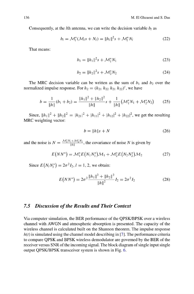
Consequently, at the lth antenna, we can write the decision variable b l as
b l = M
∗
l (M l s + N l ) = =h l
2 s + M
∗
l N l
(22)
That means:
b 1 = h 1
2 s + M
∗
1 N 1
(23)
b 2 = h 2
2 s + M
∗
2 N 2
(24)
The MRC decision variable can be written as the sum of b 1 and b 2 over the
normalized impulse response. For h 2 = (h 21 h 22 h 21 h 22 )
t , we have
b =
1
h
(b 1 + b 2 ) =
h 1
2
+ h 2
2
h
s +
1
h
M
∗
1 N 1 + M
∗
2 N 2
(25)
Since, h 1
2
+ h 2
2
= |h 21 |
2
+ |h 11 |
2
+ |h 12 |
2
+ |h 22 |
2 , we get the resulting
MRC weighting vector:
b = hs + N
(26)
and the noise is N =
M
∗
1 N 1 +M
∗
2 N 2
h
, the covariance of noise N is given by
E
N N
∗
= M
∗
1 E
N 1 N
∗
1
M 1 + M
∗
2 E
N 2 N
∗
2
M 2
(27)
Since E
N l N
∗
l
= 2σ
2 I 2 , l = 1, 2, we obtain:
E
N N
∗
= 2σ
2 h 1
2
+ h 2
2
h
2
I 2 = 2σ
2 I 2
(28)
7.5 Discussion of the Results and Their Context
Via computer simulation, the BER performance of the QPSK/BPSK over a wireless
channel with AWGN and atmospheric absorption is presented. The capacity of the
wireless channel is calculated built on the Shannon theorem. The impulse response
h(t) is simulated using the channel model describing in [7]. The performance criteria
to compare QPSK and BPSK wireless demodulator are governed by the BER of the
receiver versus SNR of the incoming signal. The block diagram of single input single
output QPSK/BPSK transceiver system is shown in Fig. 6.
M. El Ghzaoui and S. Das
Consequently, at the lth antenna, we can write the decision variable b l as
b l = M
∗
l (M l s + N l ) = =h l
2 s + M
∗
l N l
(22)
That means:
b 1 = h 1
2 s + M
∗
1 N 1
(23)
b 2 = h 2
2 s + M
∗
2 N 2
(24)
The MRC decision variable can be written as the sum of b 1 and b 2 over the
normalized impulse response. For h 2 = (h 21 h 22 h 21 h 22 )
t , we have
b =
1
h
(b 1 + b 2 ) =
h 1
2
+ h 2
2
h
s +
1
h
M
∗
1 N 1 + M
∗
2 N 2
(25)
Since, h 1
2
+ h 2
2
= |h 21 |
2
+ |h 11 |
2
+ |h 12 |
2
+ |h 22 |
2 , we get the resulting
MRC weighting vector:
b = hs + N
(26)
and the noise is N =
M
∗
1 N 1 +M
∗
2 N 2
h
, the covariance of noise N is given by
E
N N
∗
= M
∗
1 E
N 1 N
∗
1
M 1 + M
∗
2 E
N 2 N
∗
2
M 2
(27)
Since E
N l N
∗
l
= 2σ
2 I 2 , l = 1, 2, we obtain:
E
N N
∗
= 2σ
2 h 1
2
+ h 2
2
h
2
I 2 = 2σ
2 I 2
(28)
7.5 Discussion of the Results and Their Context
Via computer simulation, the BER performance of the QPSK/BPSK over a wireless
channel with AWGN and atmospheric absorption is presented. The capacity of the
wireless channel is calculated built on the Shannon theorem. The impulse response
h(t) is simulated using the channel model describing in [7]. The performance criteria
to compare QPSK and BPSK wireless demodulator are governed by the BER of the
receiver versus SNR of the incoming signal. The block diagram of single input single
output QPSK/BPSK transceiver system is shown in Fig. 6.