

166
K. Kamada et al.
0.075
0.08
0.085
0.09
0.095
0.1
0.105
0.11
0
50
100
150
200
Binomial sum
Gaussian approx.
R
1D
(200, n
lag
)
n lag
0
0.01
0.02
0.03
0.04
0.05
0.06
0
50
100
150
200
250
R 1D (530,n lag )
R 2D
(310,n lag
,0)
R 2D
(310,n lag
,0.87)
R
mD
(n
lag
)
n lag
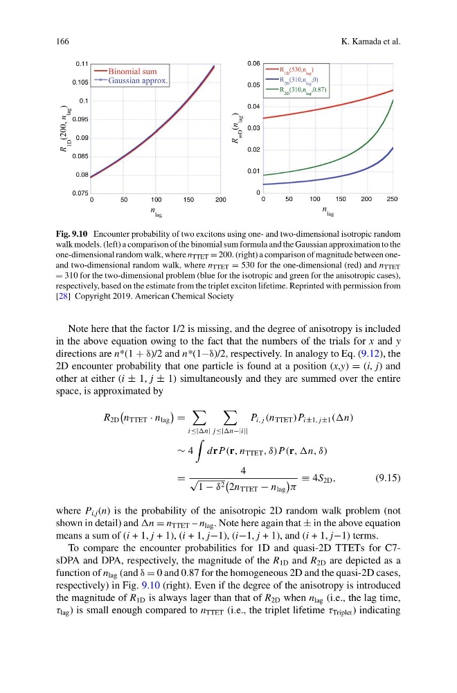
Fig. 9.10 Encounter probability of two excitons using one- and two-dimensional isotropic random
walk models. (left) a comparison of the binomial sum formula and the Gaussian approximation to the
one-dimensional random walk, where n TTET = 200. (right) a comparison of magnitude between oneand two-dimensional random walk, where n TTET = 530 for the one-dimensional (red) and n TTET
= 310 for the two-dimensional problem (blue for the isotropic and green for the anisotropic cases),
respectively, based on the estimate from the triplet exciton lifetime. Reprinted with permission from
[28] Copyright 2019. American Chemical Society
Note here that the factor 1/2 is missing, and the degree of anisotropy is included
in the above equation owing to the fact that the numbers of the trials for x and y
directions are n*(1 + δ)/2 and n*(1−δ)/2, respectively. In analogy to Eq. (9.12), the
2D encounter probability that one particle is found at a position (x,y) = (i, j) and
other at either (i ± 1, j ± 1) simultaneously and they are summed over the entire
space, is approximated by
R 2D
n TTET · n lag
=
i≤|
j≤|
P i, j (n TTET )P i±1, j±1 (
∼ 4
dr P(r, n TTET , δ)P(r, ,n, δ)
=
4
√
1 − δ 2
2n TTET − n lag
π
≡ 4S 2D ,
(9.15)
where P i,j (n) is the probability of the anisotropic 2D random walk problem (not
shown in detail) and = n TTET – n lag . Note here again that ± in the above equation
means a sum of (i + 1, j + 1), (i + 1, j−1), (i−1, j + 1), and (i + 1, j−1) terms.
To compare the encounter probabilities for 1D and quasi-2D TTETs for C7sDPA and DPA, respectively, the magnitude of the R 1D and R 2D are depicted as a
function of n lag (and δ = 0 and 0.87 for the homogeneous 2D and the quasi-2D cases,
respectively) in Fig. 9.10 (right). Even if the degree of the anisotropy is introduced
the magnitude of R 1D is always lager than that of R 2D when n lag (i.e., the lag time,
τ lag ) is small enough compared to n TTET (i.e., the triplet lifetime τ Triplet ) indicating
K. Kamada et al.
0.075
0.08
0.085
0.09
0.095
0.1
0.105
0.11
0
50
100
150
200
Binomial sum
Gaussian approx.
R
1D
(200, n
lag
)
n lag
0
0.01
0.02
0.03
0.04
0.05
0.06
0
50
100
150
200
250
R 1D (530,n lag )
R 2D
(310,n lag
,0)
R 2D
(310,n lag
,0.87)
R
mD
(n
lag
)
n lag
Fig. 9.10 Encounter probability of two excitons using one- and two-dimensional isotropic random
walk models. (left) a comparison of the binomial sum formula and the Gaussian approximation to the
one-dimensional random walk, where n TTET = 200. (right) a comparison of magnitude between oneand two-dimensional random walk, where n TTET = 530 for the one-dimensional (red) and n TTET
= 310 for the two-dimensional problem (blue for the isotropic and green for the anisotropic cases),
respectively, based on the estimate from the triplet exciton lifetime. Reprinted with permission from
[28] Copyright 2019. American Chemical Society
Note here that the factor 1/2 is missing, and the degree of anisotropy is included
in the above equation owing to the fact that the numbers of the trials for x and y
directions are n*(1 + δ)/2 and n*(1−δ)/2, respectively. In analogy to Eq. (9.12), the
2D encounter probability that one particle is found at a position (x,y) = (i, j) and
other at either (i ± 1, j ± 1) simultaneously and they are summed over the entire
space, is approximated by
R 2D
n TTET · n lag
=
i≤|
j≤|
P i, j (n TTET )P i±1, j±1 (
∼ 4
dr P(r, n TTET , δ)P(r, ,n, δ)
=
4
√
1 − δ 2
2n TTET − n lag
π
≡ 4S 2D ,
(9.15)
where P i,j (n) is the probability of the anisotropic 2D random walk problem (not
shown in detail) and = n TTET – n lag . Note here again that ± in the above equation
means a sum of (i + 1, j + 1), (i + 1, j−1), (i−1, j + 1), and (i + 1, j−1) terms.
To compare the encounter probabilities for 1D and quasi-2D TTETs for C7sDPA and DPA, respectively, the magnitude of the R 1D and R 2D are depicted as a
function of n lag (and δ = 0 and 0.87 for the homogeneous 2D and the quasi-2D cases,
respectively) in Fig. 9.10 (right). Even if the degree of the anisotropy is introduced
the magnitude of R 1D is always lager than that of R 2D when n lag (i.e., the lag time,
τ lag ) is small enough compared to n TTET (i.e., the triplet lifetime τ Triplet ) indicating