

102
R. S. Stankovi´ c et al.
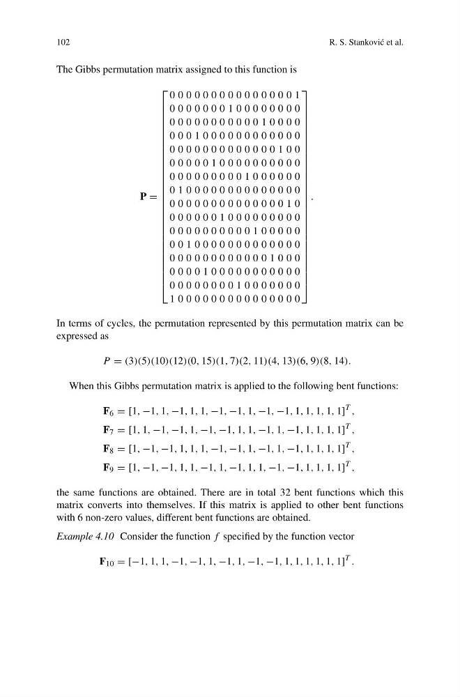
The Gibbs permutation matrix assigned to this function is
P =
⎡
⎢
⎢
⎢
⎢
⎢
⎢
⎢
⎢
⎢
⎢
⎢
⎢
⎢
⎢
⎢
⎢
⎢
⎢
⎢
⎢
⎢
⎢
⎢
⎢
⎢
⎢
⎢
⎢
⎣
0 0 0 0 0 0 0 0 0 0 0 0 0 0 0 1
0 0 0 0 0 0 0 1 0 0 0 0 0 0 0 0
0 0 0 0 0 0 0 0 0 0 0 1 0 0 0 0
0 0 0 1 0 0 0 0 0 0 0 0 0 0 0 0
0 0 0 0 0 0 0 0 0 0 0 0 0 1 0 0
0 0 0 0 0 1 0 0 0 0 0 0 0 0 0 0
0 0 0 0 0 0 0 0 0 1 0 0 0 0 0 0
0 1 0 0 0 0 0 0 0 0 0 0 0 0 0 0
0 0 0 0 0 0 0 0 0 0 0 0 0 0 1 0
0 0 0 0 0 0 1 0 0 0 0 0 0 0 0 0
0 0 0 0 0 0 0 0 0 0 1 0 0 0 0 0
0 0 1 0 0 0 0 0 0 0 0 0 0 0 0 0
0 0 0 0 0 0 0 0 0 0 0 0 1 0 0 0
0 0 0 0 1 0 0 0 0 0 0 0 0 0 0 0
0 0 0 0 0 0 0 0 1 0 0 0 0 0 0 0
1 0 0 0 0 0 0 0 0 0 0 0 0 0 0 0
⎤
⎥
⎥
⎥
⎥
⎥
⎥
⎥
⎥
⎥
⎥
⎥
⎥
⎥
⎥
⎥
⎥
⎥
⎥
⎥
⎥
⎥
⎥
⎥
⎥
⎥
⎥
⎥
⎥
⎦
.
In terms of cycles, the permutation represented by this permutation matrix can be
expressed as
P = (3)(5)(10)(12)(0, 15)(1, 7)(2, 11)(4, 13)(6, 9)(8, 14).
When this Gibbs permutation matrix is applied to the following bent functions:
F 6 = [1, −1, 1, −1, 1, 1, −1, −1, 1, −1, −1, 1, 1, 1, 1, 1]
T ,
F 7 = [1, 1, −1, −1, 1, −1, −1, 1, 1, −1, 1, −1, 1, 1, 1, 1]
T ,
F 8 = [1, −1, −1, 1, 1, 1, −1, −1, 1, −1, 1, −1, 1, 1, 1, 1]
T ,
F 9 = [1, −1, −1, 1, 1, −1, 1, −1, 1, 1, −1, −1, 1, 1, 1, 1]
T ,
the same functions are obtained. There are in total 32 bent functions which this
matrix converts into themselves. If this matrix is applied to other bent functions
with 6 non-zero values, different bent functions are obtained.
Example 4.10 Consider the function f specified by the function vector
F 10 = [−1, 1, 1, −1, −1, 1, −1, 1, −1, −1, 1, 1, 1, 1, 1, 1]
T .
R. S. Stankovi´ c et al.
The Gibbs permutation matrix assigned to this function is
P =
⎡
⎢
⎢
⎢
⎢
⎢
⎢
⎢
⎢
⎢
⎢
⎢
⎢
⎢
⎢
⎢
⎢
⎢
⎢
⎢
⎢
⎢
⎢
⎢
⎢
⎢
⎢
⎢
⎢
⎣
0 0 0 0 0 0 0 0 0 0 0 0 0 0 0 1
0 0 0 0 0 0 0 1 0 0 0 0 0 0 0 0
0 0 0 0 0 0 0 0 0 0 0 1 0 0 0 0
0 0 0 1 0 0 0 0 0 0 0 0 0 0 0 0
0 0 0 0 0 0 0 0 0 0 0 0 0 1 0 0
0 0 0 0 0 1 0 0 0 0 0 0 0 0 0 0
0 0 0 0 0 0 0 0 0 1 0 0 0 0 0 0
0 1 0 0 0 0 0 0 0 0 0 0 0 0 0 0
0 0 0 0 0 0 0 0 0 0 0 0 0 0 1 0
0 0 0 0 0 0 1 0 0 0 0 0 0 0 0 0
0 0 0 0 0 0 0 0 0 0 1 0 0 0 0 0
0 0 1 0 0 0 0 0 0 0 0 0 0 0 0 0
0 0 0 0 0 0 0 0 0 0 0 0 1 0 0 0
0 0 0 0 1 0 0 0 0 0 0 0 0 0 0 0
0 0 0 0 0 0 0 0 1 0 0 0 0 0 0 0
1 0 0 0 0 0 0 0 0 0 0 0 0 0 0 0
⎤
⎥
⎥
⎥
⎥
⎥
⎥
⎥
⎥
⎥
⎥
⎥
⎥
⎥
⎥
⎥
⎥
⎥
⎥
⎥
⎥
⎥
⎥
⎥
⎥
⎥
⎥
⎥
⎥
⎦
.
In terms of cycles, the permutation represented by this permutation matrix can be
expressed as
P = (3)(5)(10)(12)(0, 15)(1, 7)(2, 11)(4, 13)(6, 9)(8, 14).
When this Gibbs permutation matrix is applied to the following bent functions:
F 6 = [1, −1, 1, −1, 1, 1, −1, −1, 1, −1, −1, 1, 1, 1, 1, 1]
T ,
F 7 = [1, 1, −1, −1, 1, −1, −1, 1, 1, −1, 1, −1, 1, 1, 1, 1]
T ,
F 8 = [1, −1, −1, 1, 1, 1, −1, −1, 1, −1, 1, −1, 1, 1, 1, 1]
T ,
F 9 = [1, −1, −1, 1, 1, −1, 1, −1, 1, 1, −1, −1, 1, 1, 1, 1]
T ,
the same functions are obtained. There are in total 32 bent functions which this
matrix converts into themselves. If this matrix is applied to other bent functions
with 6 non-zero values, different bent functions are obtained.
Example 4.10 Consider the function f specified by the function vector
F 10 = [−1, 1, 1, −1, −1, 1, −1, 1, −1, −1, 1, 1, 1, 1, 1, 1]
T .