

52
4 Examples of Classical Mechanical Projections
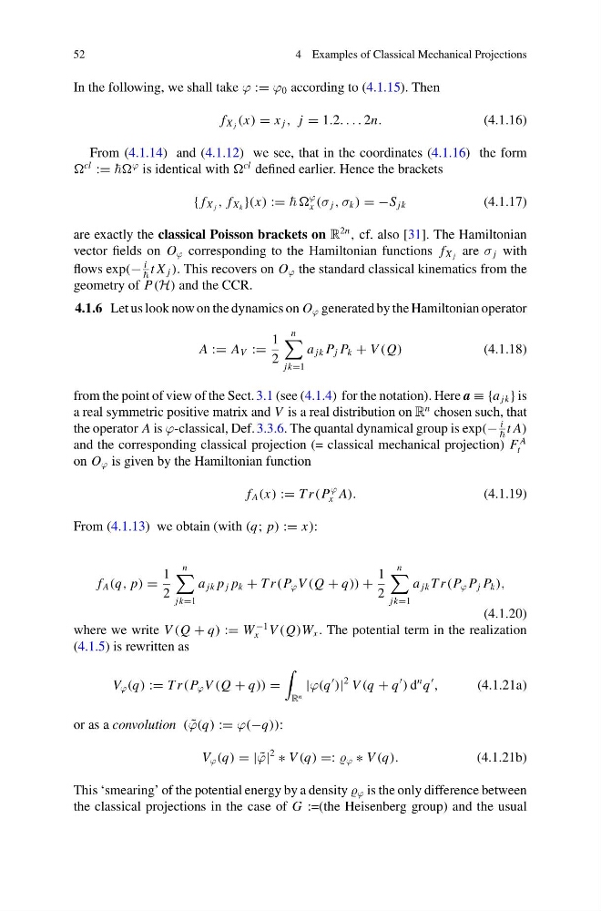
In the following, we shall take ϕ := ϕ 0 according to (4.1.15). Then
f X j (x) = x j , j = 1.2. . . . 2n.
(4.1.16)
From (4.1.14) and (4.1.12) we see, that in the coordinates (4.1.16) the form
cl
:=
ϕ is identical with
cl defined earlier. Hence the brackets
{ f X j , f X k }(x) :=
ϕ
x (σ j , σ k ) = −S jk
(4.1.17)
are exactly the classical Poisson brackets on R
2n
, cf. also [31]. The Hamiltonian
vector fields on O ϕ corresponding to the Hamiltonian functions f X j are σ j with
flows exp(−
i
t X j ). This recovers on O ϕ the standard classical kinematics from the
geometry of P(H) and the CCR.
4.1.6 Let us look now on the dynamics on O ϕ generated by the Hamiltonian operator
A := A V :=
1
2
n
jk=1
a jk P j P k + V (Q)
(4.1.18)
from the point of view of the Sect. 3.1 (see (4.1.4) for the notation). Here a ≡ {a jk } is
a real symmetric positive matrix and V is a real distribution on R
n chosen such, that
the operator A is ϕ-classical, Def. 3.3.6. The quantal dynamical group is exp(−
i
t A)
and the corresponding classical projection (= classical mechanical projection) F
A
t
on O ϕ is given by the Hamiltonian function
f A (x) := T r(P
ϕ
x A).
(4.1.19)
From (4.1.13) we obtain (with (q; p) := x):
f A (q, p) =
1
2
n
jk=1
a jk p j p k + T r(P ϕ V (Q + q)) +
1
2
n
jk=1
a jk T r(P ϕ P j P k ),
(4.1.20)
where we write V (Q + q) := W
−1
x V (Q)W x . The potential term in the realization
(4.1.5) is rewritten as
V ϕ (q) := T r(P ϕ V (Q + q)) =
R n
|ϕ(q
)|
2 V (q + q
) d
n q
,
(4.1.21a)
or as a convolution ( ˜
ϕ(q) := ϕ(−q)):
V ϕ (q) = | ˜
ϕ|
2
∗ V (q) =: ϕ ∗ V (q).
(4.1.21b)
This ‘smearing’ of the potential energy by a density ϕ is the only difference between
the classical projections in the case of G :=(the Heisenberg group) and the usual
4 Examples of Classical Mechanical Projections
In the following, we shall take ϕ := ϕ 0 according to (4.1.15). Then
f X j (x) = x j , j = 1.2. . . . 2n.
(4.1.16)
From (4.1.14) and (4.1.12) we see, that in the coordinates (4.1.16) the form
cl
:=
ϕ is identical with
cl defined earlier. Hence the brackets
{ f X j , f X k }(x) :=
ϕ
x (σ j , σ k ) = −S jk
(4.1.17)
are exactly the classical Poisson brackets on R
2n
, cf. also [31]. The Hamiltonian
vector fields on O ϕ corresponding to the Hamiltonian functions f X j are σ j with
flows exp(−
i
t X j ). This recovers on O ϕ the standard classical kinematics from the
geometry of P(H) and the CCR.
4.1.6 Let us look now on the dynamics on O ϕ generated by the Hamiltonian operator
A := A V :=
1
2
n
jk=1
a jk P j P k + V (Q)
(4.1.18)
from the point of view of the Sect. 3.1 (see (4.1.4) for the notation). Here a ≡ {a jk } is
a real symmetric positive matrix and V is a real distribution on R
n chosen such, that
the operator A is ϕ-classical, Def. 3.3.6. The quantal dynamical group is exp(−
i
t A)
and the corresponding classical projection (= classical mechanical projection) F
A
t
on O ϕ is given by the Hamiltonian function
f A (x) := T r(P
ϕ
x A).
(4.1.19)
From (4.1.13) we obtain (with (q; p) := x):
f A (q, p) =
1
2
n
jk=1
a jk p j p k + T r(P ϕ V (Q + q)) +
1
2
n
jk=1
a jk T r(P ϕ P j P k ),
(4.1.20)
where we write V (Q + q) := W
−1
x V (Q)W x . The potential term in the realization
(4.1.5) is rewritten as
V ϕ (q) := T r(P ϕ V (Q + q)) =
R n
|ϕ(q
)|
2 V (q + q
) d
n q
,
(4.1.21a)
or as a convolution ( ˜
ϕ(q) := ϕ(−q)):
V ϕ (q) = | ˜
ϕ|
2
∗ V (q) =: ϕ ∗ V (q).
(4.1.21b)
This ‘smearing’ of the potential energy by a density ϕ is the only difference between
the classical projections in the case of G :=(the Heisenberg group) and the usual