

30
2 Geometry of the State Space of Quantum Mechanics
The functions (2.3.5) for specific x’s are differentiable if the corresponding generator A has domain D(A) containing x ∈ x : x ∈ D(A). If A ∈ L(H ), then functions
(2.3.5) are analytic in t ∈ C, ∀ x ∈ P(H). It is clear from the group property of
t → F t , that differentiability of (2.3.5) in any point x for t = 0 implies differentiability on the whole curve (2.3.5), i.e. for all t ∈ R.
2.3.5 We have obtained a set of differentiable curves lying densely in P(H) for
any one-parameter weakly continuous group F t of symmetries of (P(H), ) (since
P D(A) is dense in P(H) for any selfadjoint A). For x ∈ P D(A) (A is a generator of
F t ), the curve (2.3.5) determines a vector σ A (x) ∈ T x P(H). The set of vectors σ A (x)
is defined for x ∈ P D(A) only, and for unbounded A it is not a differentiable vector
field on P(H) (it is differentiable only in directions of some curves lying densely in
P D(A), and in P(H)). We shall call it, nevertheless, ‘the vector field σ A ’. Its value
in x is expressed in [x]
⊥ according to (2.1.16) :
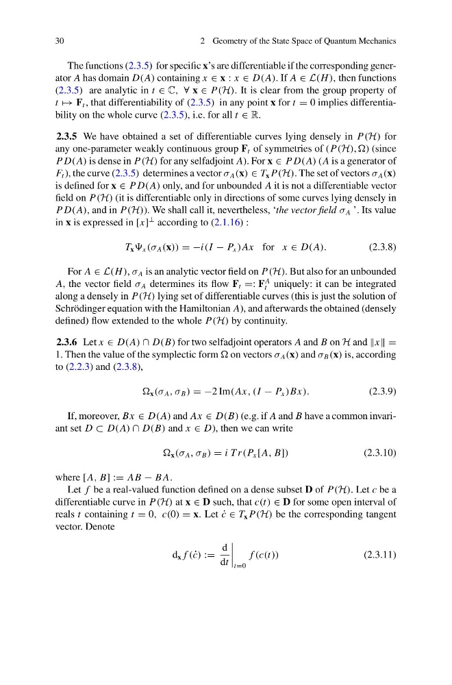
T x x (σ A (x)) = −i(I − P x )Ax for x ∈ D(A).
(2.3.8)
For A ∈ L(H ), σ A is an analytic vector field on P(H). But also for an unbounded
A, the vector field σ A determines its flow F t =: F
A
t uniquely: it can be integrated
along a densely in P(H) lying set of differentiable curves (this is just the solution of
Schrödinger equation with the Hamiltonian A), and afterwards the obtained (densely
defined) flow extended to the whole P(H) by continuity.
2.3.6 Let x ∈ D(A) ∩ D(B) for two selfadjoint operators A and B on H and x =
1. Then the value of the symplectic form on vectors σ A (x) and σ B (x) is, according
to (2.2.3) and (2.3.8),
x (σ A , σ B ) = −2 Im(Ax, (I − P x )Bx).
(2.3.9)
If, moreover, Bx ∈ D(A) and Ax ∈ D(B) (e.g. if A and B have a common invariant set D ⊂ D(A) ∩ D(B) and x ∈ D), then we can write
x (σ A , σ B ) = i T r(P x [A, B])
(2.3.10)
where [A, B] := AB − B A.
Let f be a real-valued function defined on a dense subset D of P(H). Let c be a
differentiable curve in P(H) at x ∈ D such, that c(t) ∈ D for some open interval of
reals t containing t = 0, c(0) = x. Let ˙
c ∈ T x P(H) be the corresponding tangent
vector. Denote
d x f ( ˙
c) :=
d
dt
t=0
f (c(t))
(2.3.11)
2 Geometry of the State Space of Quantum Mechanics
The functions (2.3.5) for specific x’s are differentiable if the corresponding generator A has domain D(A) containing x ∈ x : x ∈ D(A). If A ∈ L(H ), then functions
(2.3.5) are analytic in t ∈ C, ∀ x ∈ P(H). It is clear from the group property of
t → F t , that differentiability of (2.3.5) in any point x for t = 0 implies differentiability on the whole curve (2.3.5), i.e. for all t ∈ R.
2.3.5 We have obtained a set of differentiable curves lying densely in P(H) for
any one-parameter weakly continuous group F t of symmetries of (P(H), ) (since
P D(A) is dense in P(H) for any selfadjoint A). For x ∈ P D(A) (A is a generator of
F t ), the curve (2.3.5) determines a vector σ A (x) ∈ T x P(H). The set of vectors σ A (x)
is defined for x ∈ P D(A) only, and for unbounded A it is not a differentiable vector
field on P(H) (it is differentiable only in directions of some curves lying densely in
P D(A), and in P(H)). We shall call it, nevertheless, ‘the vector field σ A ’. Its value
in x is expressed in [x]
⊥ according to (2.1.16) :
T x x (σ A (x)) = −i(I − P x )Ax for x ∈ D(A).
(2.3.8)
For A ∈ L(H ), σ A is an analytic vector field on P(H). But also for an unbounded
A, the vector field σ A determines its flow F t =: F
A
t uniquely: it can be integrated
along a densely in P(H) lying set of differentiable curves (this is just the solution of
Schrödinger equation with the Hamiltonian A), and afterwards the obtained (densely
defined) flow extended to the whole P(H) by continuity.
2.3.6 Let x ∈ D(A) ∩ D(B) for two selfadjoint operators A and B on H and x =
1. Then the value of the symplectic form on vectors σ A (x) and σ B (x) is, according
to (2.2.3) and (2.3.8),
x (σ A , σ B ) = −2 Im(Ax, (I − P x )Bx).
(2.3.9)
If, moreover, Bx ∈ D(A) and Ax ∈ D(B) (e.g. if A and B have a common invariant set D ⊂ D(A) ∩ D(B) and x ∈ D), then we can write
x (σ A , σ B ) = i T r(P x [A, B])
(2.3.10)
where [A, B] := AB − B A.
Let f be a real-valued function defined on a dense subset D of P(H). Let c be a
differentiable curve in P(H) at x ∈ D such, that c(t) ∈ D for some open interval of
reals t containing t = 0, c(0) = x. Let ˙
c ∈ T x P(H) be the corresponding tangent
vector. Denote
d x f ( ˙
c) :=
d
dt
t=0
f (c(t))
(2.3.11)