

200
7 Some Models of “Quantum Measurement”
t := e
−it
H
0 = c + |++ ⊗ e
−it H
0 + c − |−− ⊗ 0 .
(7.5.23)
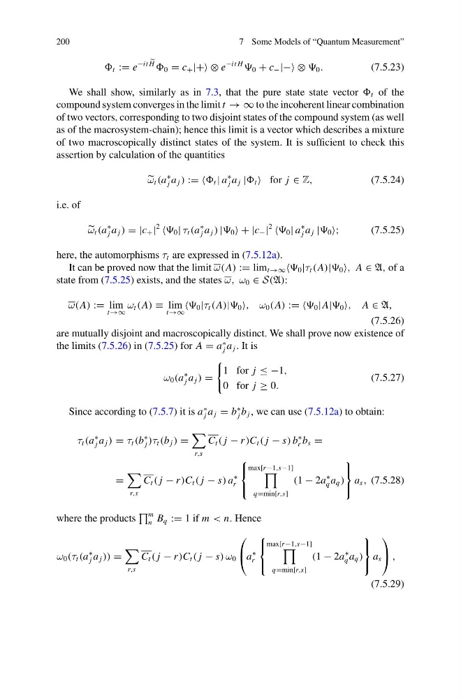
We shall show, similarly as in 7.3, that the pure state state vector t of the
compound system converges in the limit t → ∞ to the incoherent linear combination
of two vectors, corresponding to two disjoint states of the compound system (as well
as of the macrosystem-chain); hence this limit is a vector which describes a mixture
of two macroscopically distinct states of the system. It is sufficient to check this
assertion by calculation of the quantities
ω t (a
∗
j a j ) := = t | a
∗
j a j | t for j ∈ Z,
(7.5.24)
i.e. of
ω t (a
∗
j a j ) = |c + |
2
0 | τ t (a
∗
j a j ) | 0 + |c − |
2
0 | a
∗
j a j | 0 ;
(7.5.25)
here, the automorphisms τ t are expressed in (7.5.12a).
It can be proved now that the limit ω(A) := lim t→∞ 0 |τ t (A)| 0 , A ∈ A, of a
state from (7.5.25) exists, and the states ω, ω 0 ∈ S(A):
ω(A) := lim
t→∞
ω t (A) ≡ lim
t→∞
0 |τ t (A)| 0 , ω 0 (A) := = 0 |A| 0 , A ∈ A,
(7.5.26)
are mutually disjoint and macroscopically distinct. We shall prove now existence of
the limits (7.5.26) in (7.5.25) for A = a
∗
j a j . It is
ω 0 (a
∗
j a j ) =
1 for j ≤ −1,
0 for j ≥ 0.
(7.5.27)
Since according to (7.5.7) it is a
∗
j a j = b
∗
j b j , we can use (7.5.12a) to obtain:
τ t (a
∗
j a j ) = τ t (b
∗
j )τ t (b j ) =
r,s
C t ( j − r )C t ( j − s) b
∗
r b s =
=
r,s
C t ( j − r )C t ( j − s) a
∗
r
⎧
⎨
⎩
max[r −1,s−1]
q=min[r,s]
(1 − 2a
∗
q a q )
⎫
⎬
⎭
a s , (7.5.28)
where the products
m
n B q := 1 if m < n. Hence
ω 0 (τ t (a
∗
j a j )) =
r,s
C t ( j − r )C t ( j − s) ω 0
⎛
⎝ a
∗
r
⎧
⎨
⎩
max[r −1,s−1]
q=min[r,s]
(1 − 2a
∗
q a q )
⎫
⎬
⎭
a s
⎞
⎠ ,
(7.5.29)
7 Some Models of “Quantum Measurement”
t := e
−it
H
0 = c + |++ ⊗ e
−it H
0 + c − |−− ⊗ 0 .
(7.5.23)
We shall show, similarly as in 7.3, that the pure state state vector t of the
compound system converges in the limit t → ∞ to the incoherent linear combination
of two vectors, corresponding to two disjoint states of the compound system (as well
as of the macrosystem-chain); hence this limit is a vector which describes a mixture
of two macroscopically distinct states of the system. It is sufficient to check this
assertion by calculation of the quantities
ω t (a
∗
j a j ) := = t | a
∗
j a j | t for j ∈ Z,
(7.5.24)
i.e. of
ω t (a
∗
j a j ) = |c + |
2
0 | τ t (a
∗
j a j ) | 0 + |c − |
2
0 | a
∗
j a j | 0 ;
(7.5.25)
here, the automorphisms τ t are expressed in (7.5.12a).
It can be proved now that the limit ω(A) := lim t→∞ 0 |τ t (A)| 0 , A ∈ A, of a
state from (7.5.25) exists, and the states ω, ω 0 ∈ S(A):
ω(A) := lim
t→∞
ω t (A) ≡ lim
t→∞
0 |τ t (A)| 0 , ω 0 (A) := = 0 |A| 0 , A ∈ A,
(7.5.26)
are mutually disjoint and macroscopically distinct. We shall prove now existence of
the limits (7.5.26) in (7.5.25) for A = a
∗
j a j . It is
ω 0 (a
∗
j a j ) =
1 for j ≤ −1,
0 for j ≥ 0.
(7.5.27)
Since according to (7.5.7) it is a
∗
j a j = b
∗
j b j , we can use (7.5.12a) to obtain:
τ t (a
∗
j a j ) = τ t (b
∗
j )τ t (b j ) =
r,s
C t ( j − r )C t ( j − s) b
∗
r b s =
=
r,s
C t ( j − r )C t ( j − s) a
∗
r
⎧
⎨
⎩
max[r −1,s−1]
q=min[r,s]
(1 − 2a
∗
q a q )
⎫
⎬
⎭
a s , (7.5.28)
where the products
m
n B q := 1 if m < n. Hence
ω 0 (τ t (a
∗
j a j )) =
r,s
C t ( j − r )C t ( j − s) ω 0
⎛
⎝ a
∗
r
⎧
⎨
⎩
max[r −1,s−1]
q=min[r,s]
(1 − 2a
∗
q a q )
⎫
⎬
⎭
a s
⎞
⎠ ,
(7.5.29)