

176
7 Some Models of “Quantum Measurement”
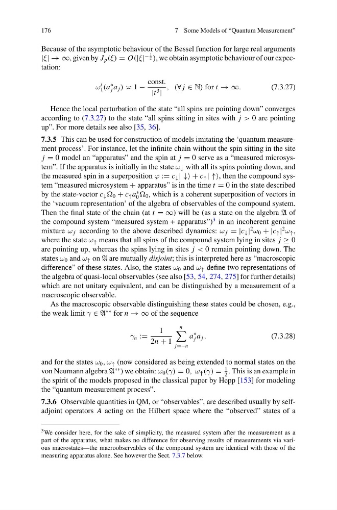
Because of the asymptotic behaviour of the Bessel function for large real arguments
|ξ| → ∞, given by J p (ξ) = O(|ξ|
−
1
2 ), we obtain asymptotic behaviour of our expectation:
ω
t
1 (a
∗
j a j ) 1 −
const.
|t 3 |
, (∀ j ∈ N) for t → ∞.
(7.3.27)
Hence the local perturbation of the state “all spins are pointing down” converges
according to (7.3.27) to the state “all spins sitting in sites with j > 0 are pointing
up”. For more details see also [35, 36].
7.3.5 This can be used for construction of models imitating the ‘quantum measurement process’. For instance, let the infinite chain without the spin sitting in the site
j = 0 model an “apparatus” and the spin at j = 0 serve as a “measured microsystem”. If the apparatus is initially in the state ω ↓ with all its spins pointing down, and
the measured spin in a superposition ϕ := c ↓ | ↓↓ + c ↑ | ↑↑, then the compound system “measured microsystem + apparatus” is in the time t = 0 in the state described
by the state-vector c ↓ 0 + c ↑ a
∗
0 0 , which is a coherent superposition of vectors in
the ‘vacuum representation’ of the algebra of observables of the compound system.
Then the final state of the chain (at t = ∞) will be (as a state on the algebra A of
the compound system “measured system + apparatus”)
3 in an incoherent genuine
mixture ω f according to the above described dynamics: ω f = |c ↓ |
2
ω 0 + |c ↑ |
2
ω ↑ ,
where the state ω ↑ means that all spins of the compound system lying in sites j ≥ 0
are pointing up, whereas the spins lying in sites j < 0 remain pointing down. The
states ω 0 and ω ↑ on A are mutually disjoint; this is interpreted here as “macroscopic
difference” of these states. Also, the states ω 0 and ω ↑ define two representations of
the algebra of quasi-local observables (see also [53, 54, 274, 275] for further details)
which are not unitary equivalent, and can be distinguished by a measurement of a
macroscopic observable.
As the macroscopic observable distinguishing these states could be chosen, e.g.,
the weak limit γ ∈ A
∗∗ for n → ∞ of the sequence
γ n :=
1
2n + 1
n
j=−n
a
∗
j a j ,
(7.3.28)
and for the states ω 0 , ω ↑ (now considered as being extended to normal states on the
von Neumann algebra A
∗∗ ) we obtain: ω 0 (γ) = 0, ω ↑ (γ) =
1
2
. This is an example in
the spirit of the models proposed in the classical paper by Hepp [153] for modeling
the “quantum measurement process”.
7.3.6 Observable quantities in QM, or “observables”, are described usually by selfadjoint operators A acting on the Hilbert space where the “observed” states of a
3 We consider here, for the sake of simplicity, the measured system after the measurement as a
part of the apparatus, what makes no difference for observing results of measurements via various macrostates—the macroobservables of the compound system are identical with those of the
measuring apparatus alone. See however the Sect. 7.3.7 below.
7 Some Models of “Quantum Measurement”
Because of the asymptotic behaviour of the Bessel function for large real arguments
|ξ| → ∞, given by J p (ξ) = O(|ξ|
−
1
2 ), we obtain asymptotic behaviour of our expectation:
ω
t
1 (a
∗
j a j ) 1 −
const.
|t 3 |
, (∀ j ∈ N) for t → ∞.
(7.3.27)
Hence the local perturbation of the state “all spins are pointing down” converges
according to (7.3.27) to the state “all spins sitting in sites with j > 0 are pointing
up”. For more details see also [35, 36].
7.3.5 This can be used for construction of models imitating the ‘quantum measurement process’. For instance, let the infinite chain without the spin sitting in the site
j = 0 model an “apparatus” and the spin at j = 0 serve as a “measured microsystem”. If the apparatus is initially in the state ω ↓ with all its spins pointing down, and
the measured spin in a superposition ϕ := c ↓ | ↓↓ + c ↑ | ↑↑, then the compound system “measured microsystem + apparatus” is in the time t = 0 in the state described
by the state-vector c ↓ 0 + c ↑ a
∗
0 0 , which is a coherent superposition of vectors in
the ‘vacuum representation’ of the algebra of observables of the compound system.
Then the final state of the chain (at t = ∞) will be (as a state on the algebra A of
the compound system “measured system + apparatus”)
3 in an incoherent genuine
mixture ω f according to the above described dynamics: ω f = |c ↓ |
2
ω 0 + |c ↑ |
2
ω ↑ ,
where the state ω ↑ means that all spins of the compound system lying in sites j ≥ 0
are pointing up, whereas the spins lying in sites j < 0 remain pointing down. The
states ω 0 and ω ↑ on A are mutually disjoint; this is interpreted here as “macroscopic
difference” of these states. Also, the states ω 0 and ω ↑ define two representations of
the algebra of quasi-local observables (see also [53, 54, 274, 275] for further details)
which are not unitary equivalent, and can be distinguished by a measurement of a
macroscopic observable.
As the macroscopic observable distinguishing these states could be chosen, e.g.,
the weak limit γ ∈ A
∗∗ for n → ∞ of the sequence
γ n :=
1
2n + 1
n
j=−n
a
∗
j a j ,
(7.3.28)
and for the states ω 0 , ω ↑ (now considered as being extended to normal states on the
von Neumann algebra A
∗∗ ) we obtain: ω 0 (γ) = 0, ω ↑ (γ) =
1
2
. This is an example in
the spirit of the models proposed in the classical paper by Hepp [153] for modeling
the “quantum measurement process”.
7.3.6 Observable quantities in QM, or “observables”, are described usually by selfadjoint operators A acting on the Hilbert space where the “observed” states of a
3 We consider here, for the sake of simplicity, the measured system after the measurement as a
part of the apparatus, what makes no difference for observing results of measurements via various macrostates—the macroobservables of the compound system are identical with those of the
measuring apparatus alone. See however the Sect. 7.3.7 below.