

8
1 Introduction
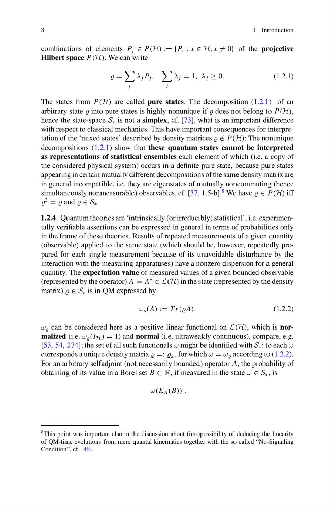
combinations of elements P j ∈ P(H) := {P x : x ∈ H, x = 0} of the projective
Hilbert space P(H). We can write
=
j
λ j P j ,
j
λ j = 1, λ j ≥ 0.
(1.2.1)
The states from P(H) are called pure states. The decomposition (1.2.1) of an
arbitrary state into pure states is highly nonunique if does not belong to P(H),
hence the state-space S ∗ is not a simplex, cf. [73], what is an important difference
with respect to classical mechanics. This have important consequences for interpretation of the ‘mixed states’ described by density matrices /
∈ P(H): The nonunique
decompositions (1.2.1) show that these quantum states cannot be interpreted
as representations of statistical ensembles each element of which (i.e. a copy of
the considered physical system) occurs in a definite pure state, because pure states
appearing in certain mutually different decompositions of the same density matrix are
in general incompatible, i.e. they are eigenstates of mutually noncommuting (hence
simultaneously nonmeasurable) observables, cf. [37, 1.5-b].
8 We have ∈ P(H) iff
2
= and ∈ S ∗ .
1.2.4 Quantum theories are ‘intrinsically (or irreducibly) statistical’, i.e. experimentally verifiable assertions can be expressed in general in terms of probabilities only
in the frame of these theories. Results of repeated measurements of a given quantity
(observable) applied to the same state (which should be, however, repeatedly prepared for each single measurement because of its unavoidable disturbance by the
interaction with the measuring apparatuses) have a nonzero dispersion for a general
quantity. The expectation value of measured values of a given bounded observable
(represented by the operator) A = A
∗
∈ L(H) in the state (represented by the density
matrix) ∈ S ∗ is in QM expressed by
ω (A) := T r(A).
(1.2.2)
ω can be considered here as a positive linear functional on L(H), which is normalized (i.e. ω (I H ) = 1) and normal (i.e. ultraweakly continuous), compare, e.g.
[53, 54, 274]; the set of all such functionals ω might be identified with S ∗ : to each ω
corresponds a unique density matrix =: ω , for which ω = ω according to (1.2.2).
For an arbitrary selfadjoint (not necessarily bounded) operator A, the probability of
obtaining of its value in a Borel set B ⊂ R, if measured in the state ω ∈ S ∗ , is
ω(E A (B)) .
8 This point was important also in the discussion about (im-)possibility of deducing the linearity
of QM-time evolutions from mere quantal kinematics together with the so called “No-Signaling
Condition”, cf. [46].
1 Introduction
combinations of elements P j ∈ P(H) := {P x : x ∈ H, x = 0} of the projective
Hilbert space P(H). We can write
=
j
λ j P j ,
j
λ j = 1, λ j ≥ 0.
(1.2.1)
The states from P(H) are called pure states. The decomposition (1.2.1) of an
arbitrary state into pure states is highly nonunique if does not belong to P(H),
hence the state-space S ∗ is not a simplex, cf. [73], what is an important difference
with respect to classical mechanics. This have important consequences for interpretation of the ‘mixed states’ described by density matrices /
∈ P(H): The nonunique
decompositions (1.2.1) show that these quantum states cannot be interpreted
as representations of statistical ensembles each element of which (i.e. a copy of
the considered physical system) occurs in a definite pure state, because pure states
appearing in certain mutually different decompositions of the same density matrix are
in general incompatible, i.e. they are eigenstates of mutually noncommuting (hence
simultaneously nonmeasurable) observables, cf. [37, 1.5-b].
8 We have ∈ P(H) iff
2
= and ∈ S ∗ .
1.2.4 Quantum theories are ‘intrinsically (or irreducibly) statistical’, i.e. experimentally verifiable assertions can be expressed in general in terms of probabilities only
in the frame of these theories. Results of repeated measurements of a given quantity
(observable) applied to the same state (which should be, however, repeatedly prepared for each single measurement because of its unavoidable disturbance by the
interaction with the measuring apparatuses) have a nonzero dispersion for a general
quantity. The expectation value of measured values of a given bounded observable
(represented by the operator) A = A
∗
∈ L(H) in the state (represented by the density
matrix) ∈ S ∗ is in QM expressed by
ω (A) := T r(A).
(1.2.2)
ω can be considered here as a positive linear functional on L(H), which is normalized (i.e. ω (I H ) = 1) and normal (i.e. ultraweakly continuous), compare, e.g.
[53, 54, 274]; the set of all such functionals ω might be identified with S ∗ : to each ω
corresponds a unique density matrix =: ω , for which ω = ω according to (1.2.2).
For an arbitrary selfadjoint (not necessarily bounded) operator A, the probability of
obtaining of its value in a Borel set B ⊂ R, if measured in the state ω ∈ S ∗ , is
ω(E A (B)) .
8 This point was important also in the discussion about (im-)possibility of deducing the linearity
of QM-time evolutions from mere quantal kinematics together with the so called “No-Signaling
Condition”, cf. [46].