

6.5 An Example: The B.C.S. Model of Superconductivity
161
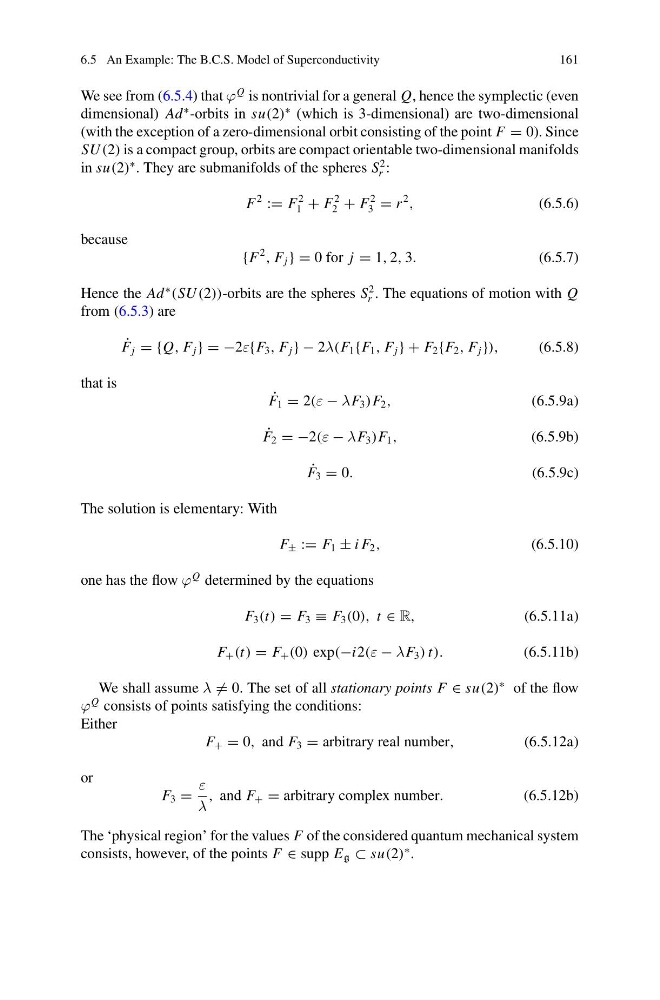
We see from (6.5.4) that ϕ
Q is nontrivial for a general Q, hence the symplectic (even
dimensional) Ad
∗ -orbits in su(2)
∗ (which is 3-dimensional) are two-dimensional
(with the exception of a zero-dimensional orbit consisting of the point F = 0). Since
SU (2) is a compact group, orbits are compact orientable two-dimensional manifolds
in su(2)
∗ . They are submanifolds of the spheres S
2
r :
F
2
:= F
2
1 + F
2
2 + F
2
3 = r
2
,
(6.5.6)
because
{F
2
, F j } = 0 for j = 1, 2, 3.
(6.5.7)
Hence the Ad
∗
(SU (2))-orbits are the spheres S
2
r . The equations of motion with Q
from (6.5.3) are
˙
F j = {Q, F j } = −2ε{F 3 , F j } − 2λ(F 1 {F 1 , F j } + F 2 {F 2 , F j }),
(6.5.8)
that is
˙
F 1 = 2(ε − λF 3 )F 2 ,
(6.5.9a)
˙
F 2 = −2(ε − λF 3 )F 1 ,
(6.5.9b)
˙
F 3 = 0.
(6.5.9c)
The solution is elementary: With
F ± := F 1 ± i F 2 ,
(6.5.10)
one has the flow ϕ
Q determined by the equations
F 3 (t) = F 3 ≡ F 3 (0), t ∈ R,
(6.5.11a)
F + (t) = F + (0) exp(−i2(ε − λF 3 ) t).
(6.5.11b)
We shall assume λ = 0. The set of all stationary points F ∈ su(2)
∗ of the flow
ϕ
Q consists of points satisfying the conditions:
Either
F + = 0, and F 3 = arbitrary real number,
(6.5.12a)
or
F 3 =
ε
λ
, and F + = arbitrary complex number.
(6.5.12b)
The ‘physical region’ for the values F of the considered quantum mechanical system
consists, however, of the points F ∈ supp E g ⊂ su(2)
∗ .
161
We see from (6.5.4) that ϕ
Q is nontrivial for a general Q, hence the symplectic (even
dimensional) Ad
∗ -orbits in su(2)
∗ (which is 3-dimensional) are two-dimensional
(with the exception of a zero-dimensional orbit consisting of the point F = 0). Since
SU (2) is a compact group, orbits are compact orientable two-dimensional manifolds
in su(2)
∗ . They are submanifolds of the spheres S
2
r :
F
2
:= F
2
1 + F
2
2 + F
2
3 = r
2
,
(6.5.6)
because
{F
2
, F j } = 0 for j = 1, 2, 3.
(6.5.7)
Hence the Ad
∗
(SU (2))-orbits are the spheres S
2
r . The equations of motion with Q
from (6.5.3) are
˙
F j = {Q, F j } = −2ε{F 3 , F j } − 2λ(F 1 {F 1 , F j } + F 2 {F 2 , F j }),
(6.5.8)
that is
˙
F 1 = 2(ε − λF 3 )F 2 ,
(6.5.9a)
˙
F 2 = −2(ε − λF 3 )F 1 ,
(6.5.9b)
˙
F 3 = 0.
(6.5.9c)
The solution is elementary: With
F ± := F 1 ± i F 2 ,
(6.5.10)
one has the flow ϕ
Q determined by the equations
F 3 (t) = F 3 ≡ F 3 (0), t ∈ R,
(6.5.11a)
F + (t) = F + (0) exp(−i2(ε − λF 3 ) t).
(6.5.11b)
We shall assume λ = 0. The set of all stationary points F ∈ su(2)
∗ of the flow
ϕ
Q consists of points satisfying the conditions:
Either
F + = 0, and F 3 = arbitrary real number,
(6.5.12a)
or
F 3 =
ε
λ
, and F + = arbitrary complex number.
(6.5.12b)
The ‘physical region’ for the values F of the considered quantum mechanical system
consists, however, of the points F ∈ supp E g ⊂ su(2)
∗ .