

6.3 Time Evolution in Generalized Mean-Field Theories
149
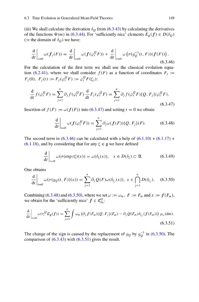
(iii) We shall calculate the derivation δ Q from (6.3.43) by calculating the derivatives
of the functions (m) in (6.3.44). For ‘sufficiently nice’ elements E g ( f ) ∈ D(δ Q )
(:= the domain of δ Q ) we have:
d
dt
t=0
ω( f t (F)) =
d
dt
t=0
ω( f (ϕ
Q
t F)) +
d
dt
t=0
ω
σ(g
−1
Q (t, F))( f (F))
.
(6.3.46)
For the calculation of the first term we shall use the classical evolution equation (6.2.41), where we shall consider f (F) as a function of coordinates F j :=
F j (0), F j (t) := F j (ϕ
Q
t F) := ϕ
Q
t F(ξ j ):
d
dt
f (ϕ
Q
t F) =
n
j=1
∂ j f (ϕ
Q
t F)
d
dt
F j (ϕ
Q
t F) =
n
j=1
∂ j f (ϕ
Q
t F){Q, F j }(ϕ
Q
t F).
(6.3.47)
Insertion of f (F) := ω( f (F)) into (6.3.47) and setting t = 0 we obtain
d
dt
t=0
ω( f (ϕ
Q
t F)) =
n
j=1
∂ j ω( f (F)){Q, F j }(F).
(6.3.48)
The second term in (6.3.46) can be calculated with a help of (6.1.10) + (6.1.17) +
(6.1.18), and by considering that for any ξ ∈ g we have defined
d
dt
t=0
ω(σ(exp tξ)(x)) = ω(δ ξ (x)), x ∈ D(δ ξ ) ⊂ A.
(6.3.49)
One obtains
d
dt
t=0
ω(σ(g Q (t, F))(x)) =
n
j=1
∂ j Q(F)ω(δ ξ j (x)), x ∈
n
j=1
D(δ ξ j ). (6.3.50)
Combining (6.3.48) and (6.3.50), where we set ω := ω m , F := F m and x := f (F m ),
we obtain for the ‘sufficiently nice’ f ∈ C
G
bs :
d
dt
t=0
ω(τ
Q
t E g ( f )) =
n
j=1
ω m
∂ j f (F m ){Q, F j }(F m ) − ∂ j Q(F m )δ ξ j ( f (F m ))
μ ω (dm).
(6.3.51)
The change of the sign is caused by the replacement of g Q by g
−1
Q in (6.3.50). The
comparison of (6.3.43) with (6.3.51) gives the result.
149
(iii) We shall calculate the derivation δ Q from (6.3.43) by calculating the derivatives
of the functions (m) in (6.3.44). For ‘sufficiently nice’ elements E g ( f ) ∈ D(δ Q )
(:= the domain of δ Q ) we have:
d
dt
t=0
ω( f t (F)) =
d
dt
t=0
ω( f (ϕ
Q
t F)) +
d
dt
t=0
ω
σ(g
−1
Q (t, F))( f (F))
.
(6.3.46)
For the calculation of the first term we shall use the classical evolution equation (6.2.41), where we shall consider f (F) as a function of coordinates F j :=
F j (0), F j (t) := F j (ϕ
Q
t F) := ϕ
Q
t F(ξ j ):
d
dt
f (ϕ
Q
t F) =
n
j=1
∂ j f (ϕ
Q
t F)
d
dt
F j (ϕ
Q
t F) =
n
j=1
∂ j f (ϕ
Q
t F){Q, F j }(ϕ
Q
t F).
(6.3.47)
Insertion of f (F) := ω( f (F)) into (6.3.47) and setting t = 0 we obtain
d
dt
t=0
ω( f (ϕ
Q
t F)) =
n
j=1
∂ j ω( f (F)){Q, F j }(F).
(6.3.48)
The second term in (6.3.46) can be calculated with a help of (6.1.10) + (6.1.17) +
(6.1.18), and by considering that for any ξ ∈ g we have defined
d
dt
t=0
ω(σ(exp tξ)(x)) = ω(δ ξ (x)), x ∈ D(δ ξ ) ⊂ A.
(6.3.49)
One obtains
d
dt
t=0
ω(σ(g Q (t, F))(x)) =
n
j=1
∂ j Q(F)ω(δ ξ j (x)), x ∈
n
j=1
D(δ ξ j ). (6.3.50)
Combining (6.3.48) and (6.3.50), where we set ω := ω m , F := F m and x := f (F m ),
we obtain for the ‘sufficiently nice’ f ∈ C
G
bs :
d
dt
t=0
ω(τ
Q
t E g ( f )) =
n
j=1
ω m
∂ j f (F m ){Q, F j }(F m ) − ∂ j Q(F m )δ ξ j ( f (F m ))
μ ω (dm).
(6.3.51)
The change of the sign is caused by the replacement of g Q by g
−1
Q in (6.3.50). The
comparison of (6.3.43) with (6.3.51) gives the result.