

One has to consider as further research how to split redundancy x into x d which
is the amount of redundancy used for fault detection and x r which is the amount of
redundancy used for recovery.
If a is inserted into equation for mean time to failure MTTF ft , we get the
following:
MTTF ft ¼
1
1 þ d c þ d r
ð
Þ1 þ 1 À cx b 1Àx
ð
Þ
ð
Þ k
ð
Þ k pf
ð4:11Þ
When we need to compare the MTTF for two systems, one with redundancy and
one without an improvement in the order of magnitude (Efficiency E, Eq. 4.12), it is
proved that the solution with redundancy introduced into the system for checking
and recovery purposes is better than the system without redundancy.
E ¼
MTTF ft
MTTF nf
ð4:12Þ
Simplified, we get the following equation for efficiency of redundancy use for
reliability gain:
E ¼
1 þ k
1 þ d c þ d r
ð
Þ1 þ 1 À cx b 1Àx
ð
Þ
ð
Þ k
ð
Þ
Figure 4.7 (upper family of functions) shows efficiency for different values of
b and x, assuming k = 100. For convenience of illustration, permanent fault ratio is
set at 10
−3 .
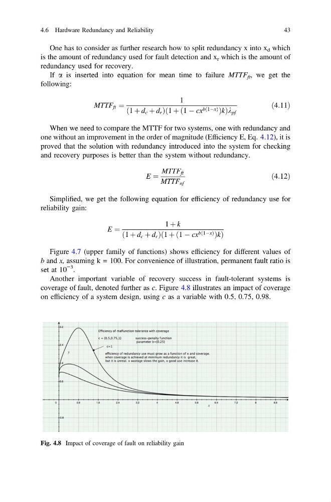
Another important variable of recovery success in fault-tolerant systems is
coverage of fault, denoted further as c. Figure 4.8 illustrates an impact of coverage
on efficiency of a system design, using c as a variable with 0.5, 0.75, 0.98.
Fig. 4.8 Impact of coverage of fault on reliability gain
4.6 Hardware Redundancy and Reliability
43
is the amount of redundancy used for fault detection and x r which is the amount of
redundancy used for recovery.
If a is inserted into equation for mean time to failure MTTF ft , we get the
following:
MTTF ft ¼
1
1 þ d c þ d r
ð
Þ1 þ 1 À cx b 1Àx
ð
Þ
ð
Þ k
ð
Þ k pf
ð4:11Þ
When we need to compare the MTTF for two systems, one with redundancy and
one without an improvement in the order of magnitude (Efficiency E, Eq. 4.12), it is
proved that the solution with redundancy introduced into the system for checking
and recovery purposes is better than the system without redundancy.
E ¼
MTTF ft
MTTF nf
ð4:12Þ
Simplified, we get the following equation for efficiency of redundancy use for
reliability gain:
E ¼
1 þ k
1 þ d c þ d r
ð
Þ1 þ 1 À cx b 1Àx
ð
Þ
ð
Þ k
ð
Þ
Figure 4.7 (upper family of functions) shows efficiency for different values of
b and x, assuming k = 100. For convenience of illustration, permanent fault ratio is
set at 10
−3 .
Another important variable of recovery success in fault-tolerant systems is
coverage of fault, denoted further as c. Figure 4.8 illustrates an impact of coverage
on efficiency of a system design, using c as a variable with 0.5, 0.75, 0.98.
Fig. 4.8 Impact of coverage of fault on reliability gain
4.6 Hardware Redundancy and Reliability
43