

What is still missing in the reliability analysis is the rate of successful recovery
a, i.e., the chance that a fault is detected successfully and the system can recover
fully from the fault. Obviously, as mentioned above, a must be in the range of (0–
1), dependent on the fault coverage c. For a, we thus introduce Eq. 4.9 with SF
being the so-called success function:
a ¼ 1 À c à SF
ð4:9Þ
This success function SF defines the recovery rate. A duplicated system can
detect all possible malfunctions and if self-checking is implemented, it can also
recover from them.
Thus, a success function should meet the following constraints, with x being the
amount of used redundancy:
– The recovery rate must be in the range of 0–1;
– If no redundancy is used x = 0, the chance for recovery is 0, and therefore
SF ! 0. If duplication is used x = 1, the recovery is in approximation 1, and
therefore SF ! 1;
– If more redundancy than duplication is used (x > 1), the system gets less
efficient.
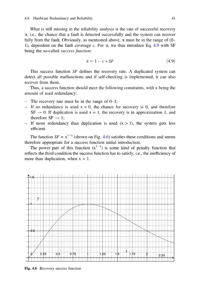
The function SF = x
1−x (shown on Fig. 4.6) satisfies these conditions and seems
therefore appropriate for a success function initial introduction.
The power part of this function (x
1−x ) is some kind of penalty function that
reflects the third condition the success function has to satisfy, i.e., the inefficiency of
more than duplication, when x > 1.
Fig. 4.6 Recovery success function
4.6 Hardware Redundancy and Reliability
41
a, i.e., the chance that a fault is detected successfully and the system can recover
fully from the fault. Obviously, as mentioned above, a must be in the range of (0–
1), dependent on the fault coverage c. For a, we thus introduce Eq. 4.9 with SF
being the so-called success function:
a ¼ 1 À c à SF
ð4:9Þ
This success function SF defines the recovery rate. A duplicated system can
detect all possible malfunctions and if self-checking is implemented, it can also
recover from them.
Thus, a success function should meet the following constraints, with x being the
amount of used redundancy:
– The recovery rate must be in the range of 0–1;
– If no redundancy is used x = 0, the chance for recovery is 0, and therefore
SF ! 0. If duplication is used x = 1, the recovery is in approximation 1, and
therefore SF ! 1;
– If more redundancy than duplication is used (x > 1), the system gets less
efficient.
The function SF = x
1−x (shown on Fig. 4.6) satisfies these conditions and seems
therefore appropriate for a success function initial introduction.
The power part of this function (x
1−x ) is some kind of penalty function that
reflects the third condition the success function has to satisfy, i.e., the inefficiency of
more than duplication, when x > 1.
Fig. 4.6 Recovery success function
4.6 Hardware Redundancy and Reliability
41