

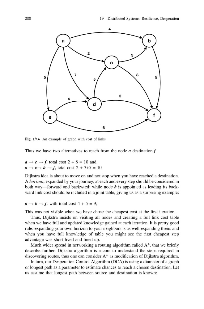
Thus we have two alternatives to reach from the node a destination f
a ! c ! f, total cost 2 + 8 = 10 and
a ! c! b ! f, total cost 2 + 3+5 = 10
Dijkstra idea is about to move on and not stop when you have reached a destination.
A horizon, expanded by your journey, at each and every step should be considered in
both way—forward and backward: while node b is appointed as leading its backward link cost should be included in a joint table, giving us as a surprising example:
a ! b ! f, with total cost 4 + 5 = 9;
This was not visible when we have chose the cheapest cost at the first iteration.
Thus, Dijkstra insists on visiting all nodes and creating a full link cost table
when we have full and updated knowledge gained at each iteration. It is pretty good
rule: expanding your own horizon to your neighbors is as well expanding theirs and
when you have full knowledge of table you might see the first cheapest step
advantage was short lived and lined up.
Much wider spread in networking a routing algorithm called A*, that we briefly
describe further. Dijkstra algorithm is a core to understand the steps required in
discovering routes, thus one can consider A* as modification of Dijkstra algorithm.
In turn, our Desperation Control Algorithm (DCA) is using a diameter of a graph
or longest path as a parameter to estimate chances to reach a chosen destination. Let
us assume that longest path between source and destination is known:
Fig. 19.4 An example of graph with cost of links
280
19 Distributed Systems: Resilience, Desperation
a ! c ! f, total cost 2 + 8 = 10 and
a ! c! b ! f, total cost 2 + 3+5 = 10
Dijkstra idea is about to move on and not stop when you have reached a destination.
A horizon, expanded by your journey, at each and every step should be considered in
both way—forward and backward: while node b is appointed as leading its backward link cost should be included in a joint table, giving us as a surprising example:
a ! b ! f, with total cost 4 + 5 = 9;
This was not visible when we have chose the cheapest cost at the first iteration.
Thus, Dijkstra insists on visiting all nodes and creating a full link cost table
when we have full and updated knowledge gained at each iteration. It is pretty good
rule: expanding your own horizon to your neighbors is as well expanding theirs and
when you have full knowledge of table you might see the first cheapest step
advantage was short lived and lined up.
Much wider spread in networking a routing algorithm called A*, that we briefly
describe further. Dijkstra algorithm is a core to understand the steps required in
discovering routes, thus one can consider A* as modification of Dijkstra algorithm.
In turn, our Desperation Control Algorithm (DCA) is using a diameter of a graph
or longest path as a parameter to estimate chances to reach a chosen destination. Let
us assume that longest path between source and destination is known:
Fig. 19.4 An example of graph with cost of links
280
19 Distributed Systems: Resilience, Desperation