

10.4 Dichotomous Recovery Algorithm
The dichotomous recovery algorithm is the second algorithm we consider in this
analysis. In fact, the only difference to the linear algorithm is the way the recovery
steps are selected. The recovery steps are no longer linearly executed, but the first
recovery step is the one with number i, and
i ¼
J
2
$ %
If the system could not be recovered (the checking logic still detects the fault
after the execution of segment J), it continues with RP i and
i ¼
J
2
þ
J
4
$
%
etc., until a correct RP is found.
This algorithm applies therefore the pattern of a binary search to find the
appropriate recovery step.
We derive now the probabilities of the events H c , H km , H kpf , H km (L), and H kpf (L)
for the dichotomous recovery. We derive P c (the probability of event H c ) as in the
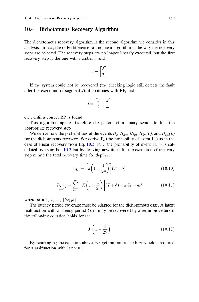
case of linear recovery from Eq. 10.2. P km (the probability of event H km ) is calculated by using Eq. 10.3 but by deriving new times for the execution of recovery
step m and the total recovery time for depth m:
t rb m ¼ k 1 À
1
2 m
$
%
T þ d
ð
Þ
ð10:10Þ
T P
m ¼
X m
i¼1
K 1 À
1
2 i
$
%
ðT þ dÞ þ md 1 À md
ð10:11Þ
where m = 1, 2, …, log 2 k
d
e.
The latency period coverage must be adapted for the dichotomous case. A latent
malfunction with a latency period l can only be recovered by a rerun procedure if
the following equation holds for m:
J 1 À
1
2 m
ð10:12Þ
By rearranging the equation above, we get minimum depth m which is required
for a malfunction with latency l
10.4 Dichotomous Recovery Algorithm
159
The dichotomous recovery algorithm is the second algorithm we consider in this
analysis. In fact, the only difference to the linear algorithm is the way the recovery
steps are selected. The recovery steps are no longer linearly executed, but the first
recovery step is the one with number i, and
i ¼
J
2
$ %
If the system could not be recovered (the checking logic still detects the fault
after the execution of segment J), it continues with RP i and
i ¼
J
2
þ
J
4
$
%
etc., until a correct RP is found.
This algorithm applies therefore the pattern of a binary search to find the
appropriate recovery step.
We derive now the probabilities of the events H c , H km , H kpf , H km (L), and H kpf (L)
for the dichotomous recovery. We derive P c (the probability of event H c ) as in the
case of linear recovery from Eq. 10.2. P km (the probability of event H km ) is calculated by using Eq. 10.3 but by deriving new times for the execution of recovery
step m and the total recovery time for depth m:
t rb m ¼ k 1 À
1
2 m
$
%
T þ d
ð
Þ
ð10:10Þ
T P
m ¼
X m
i¼1
K 1 À
1
2 i
$
%
ðT þ dÞ þ md 1 À md
ð10:11Þ
where m = 1, 2, …, log 2 k
d
e.
The latency period coverage must be adapted for the dichotomous case. A latent
malfunction with a latency period l can only be recovered by a rerun procedure if
the following equation holds for m:
J 1 À
1
2 m
ð10:12Þ
By rearranging the equation above, we get minimum depth m which is required
for a malfunction with latency l
10.4 Dichotomous Recovery Algorithm
159