

3.5 Oscillations and Waves
37
edge of a front segment propagating upwards in the picture lags behind and, as the
segment spreads out, spirals are formed at its sides. Patterns and waves on a much
finer scale (visible under an electron microscope rather than by naked eye), and
with an added anisotropy distorting round wave fronts to a squared form (Fig. 3.13,
right), were observed on catalytic surfaces and earned Gerhard Ertl the 2007 Nobel
Prize in Chemistry. Their mechanism is more complex, as it involves restructuring
the catalytic surface.
A typical pattern is a maze of spirals, as in the left-hand panel of Fig. 3.13. A
wave is characterized by its propagation direction, which is a vector rotating by
360 ◦ around the point wherefrom a circular or spiral wave originates. This point is
therefore a defect of unit charge – compare with the half-charge defects in the alignment of a director lacking an arrow (Sect. 3.3). The charge is everywhere positive:
as you go round a contour, the vector rotates in the same direction. Defects of the
same charge repel each other, which prevents the ordering of a disorganized pattern.
The formation of self-organized patterns, either stationary or oscillatory, is such a
basic and widespread phenomenon that its essential features can be imitated even by
a very simple model. This is the FitzHugh–Nagumo (FN) system (FitzHugh, 1961),
first derived as a simplified version of the nerve conduction model by Hodgkin and
Huxley (1952), which is itself a far-reaching simplification. What is essential is
to have two reaction–diffusion equations: first, a nonlinear activator equation, and
second, an inhibitor equation, which can be linear. A cubic nonlinearity suffices to
have two levels of the activator that would be stable at some level of the inhibitor
concentration.
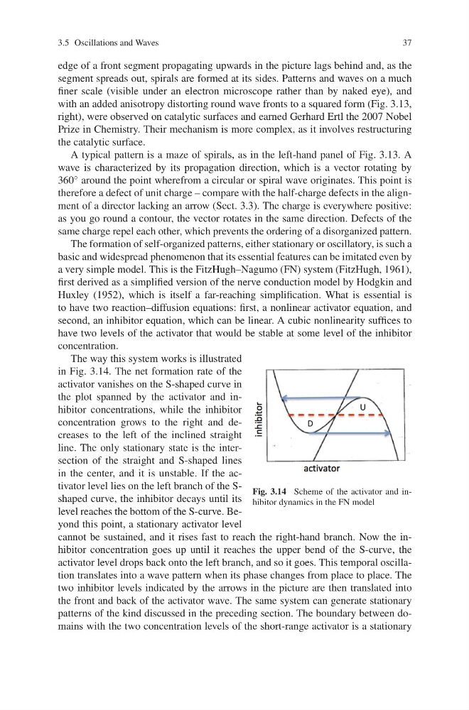
Fig. 3.14 Scheme of the activator and inhibitor dynamics in the FN model
The way this system works is illustrated
in Fig. 3.14. The net formation rate of the
activator vanishes on the S-shaped curve in
the plot spanned by the activator and inhibitor concentrations, while the inhibitor
concentration grows to the right and decreases to the left of the inclined straight
line. The only stationary state is the intersection of the straight and S-shaped lines
in the center, and it is unstable. If the activator level lies on the left branch of the Sshaped curve, the inhibitor decays until its
level reaches the bottom of the S-curve. Beyond this point, a stationary activator level
cannot be sustained, and it rises fast to reach the right-hand branch. Now the inhibitor concentration goes up until it reaches the upper bend of the S-curve, the
activator level drops back onto the left branch, and so it goes. This temporal oscillation translates into a wave pattern when its phase changes from place to place. The
two inhibitor levels indicated by the arrows in the picture are then translated into
the front and back of the activator wave. The same system can generate stationary
patterns of the kind discussed in the preceding section. The boundary between domains with the two concentration levels of the short-range activator is a stationary
37
edge of a front segment propagating upwards in the picture lags behind and, as the
segment spreads out, spirals are formed at its sides. Patterns and waves on a much
finer scale (visible under an electron microscope rather than by naked eye), and
with an added anisotropy distorting round wave fronts to a squared form (Fig. 3.13,
right), were observed on catalytic surfaces and earned Gerhard Ertl the 2007 Nobel
Prize in Chemistry. Their mechanism is more complex, as it involves restructuring
the catalytic surface.
A typical pattern is a maze of spirals, as in the left-hand panel of Fig. 3.13. A
wave is characterized by its propagation direction, which is a vector rotating by
360 ◦ around the point wherefrom a circular or spiral wave originates. This point is
therefore a defect of unit charge – compare with the half-charge defects in the alignment of a director lacking an arrow (Sect. 3.3). The charge is everywhere positive:
as you go round a contour, the vector rotates in the same direction. Defects of the
same charge repel each other, which prevents the ordering of a disorganized pattern.
The formation of self-organized patterns, either stationary or oscillatory, is such a
basic and widespread phenomenon that its essential features can be imitated even by
a very simple model. This is the FitzHugh–Nagumo (FN) system (FitzHugh, 1961),
first derived as a simplified version of the nerve conduction model by Hodgkin and
Huxley (1952), which is itself a far-reaching simplification. What is essential is
to have two reaction–diffusion equations: first, a nonlinear activator equation, and
second, an inhibitor equation, which can be linear. A cubic nonlinearity suffices to
have two levels of the activator that would be stable at some level of the inhibitor
concentration.
Fig. 3.14 Scheme of the activator and inhibitor dynamics in the FN model
The way this system works is illustrated
in Fig. 3.14. The net formation rate of the
activator vanishes on the S-shaped curve in
the plot spanned by the activator and inhibitor concentrations, while the inhibitor
concentration grows to the right and decreases to the left of the inclined straight
line. The only stationary state is the intersection of the straight and S-shaped lines
in the center, and it is unstable. If the activator level lies on the left branch of the Sshaped curve, the inhibitor decays until its
level reaches the bottom of the S-curve. Beyond this point, a stationary activator level
cannot be sustained, and it rises fast to reach the right-hand branch. Now the inhibitor concentration goes up until it reaches the upper bend of the S-curve, the
activator level drops back onto the left branch, and so it goes. This temporal oscillation translates into a wave pattern when its phase changes from place to place. The
two inhibitor levels indicated by the arrows in the picture are then translated into
the front and back of the activator wave. The same system can generate stationary
patterns of the kind discussed in the preceding section. The boundary between domains with the two concentration levels of the short-range activator is a stationary