

5.3 Shell Element Design
83
4-node
9-node
16-node
a) Lagrange family of shell elements
b) Serendipity family of shell elements
12-node
8-node
4-node
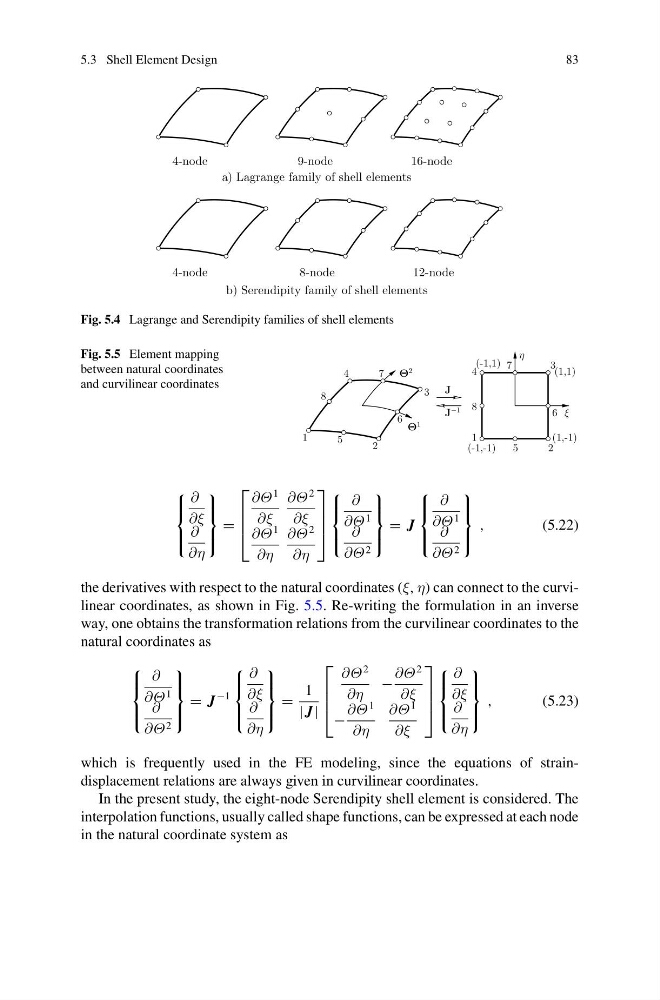
Fig. 5.4 Lagrange and Serendipity families of shell elements
Fig. 5.5 Element mapping
between natural coordinates
and curvilinear coordinates
J
J
−1
Θ
1
Θ
2
1
3
2
4
5
8
7
6
5
2
6 ξ
8
7
3
η
1
(-1,-1)
(1,-1)
(1,1)
(-1,1)
4
⎧
⎪ ⎨
⎪ ⎩
∂
∂ξ
∂
∂η
⎫
⎪ ⎬
⎪ ⎭
=
⎡
⎢
⎢
⎣
∂Θ
1
∂ξ
∂Θ
2
∂ξ
∂Θ
1
∂η
∂Θ
2
∂η
⎤
⎥
⎥
⎦
⎧
⎪ ⎨
⎪ ⎩
∂
∂Θ 1
∂
∂Θ 2
⎫
⎪ ⎬
⎪ ⎭
= J
⎧
⎪ ⎨
⎪ ⎩
∂
∂Θ 1
∂
∂Θ 2
⎫
⎪ ⎬
⎪ ⎭
,
(5.22)
the derivatives with respect to the natural coordinates (ξ, η) can connect to the curvilinear coordinates, as shown in Fig. 5.5. Re-writing the formulation in an inverse
way, one obtains the transformation relations from the curvilinear coordinates to the
natural coordinates as
⎧
⎪ ⎨
⎪ ⎩
∂
∂Θ 1
∂
∂Θ 2
⎫
⎪ ⎬
⎪ ⎭
= J
−1
⎧
⎪ ⎨
⎪ ⎩
∂
∂ξ
∂
∂η
⎫
⎪ ⎬
⎪ ⎭
=
1
| J|
⎡
⎢
⎢
⎣
∂Θ
2
∂η
−
∂Θ
2
∂ξ
−
∂Θ
1
∂η
∂Θ
1
∂ξ
⎤
⎥
⎥
⎦
⎧
⎪ ⎨
⎪ ⎩
∂
∂ξ
∂
∂η
⎫
⎪ ⎬
⎪ ⎭
,
(5.23)
which is frequently used in the FE modeling, since the equations of straindisplacement relations are always given in curvilinear coordinates.
In the present study, the eight-node Serendipity shell element is considered. The
interpolation functions, usually called shape functions, can be expressed at each node
in the natural coordinate system as
83
4-node
9-node
16-node
a) Lagrange family of shell elements
b) Serendipity family of shell elements
12-node
8-node
4-node
Fig. 5.4 Lagrange and Serendipity families of shell elements
Fig. 5.5 Element mapping
between natural coordinates
and curvilinear coordinates
J
J
−1
Θ
1
Θ
2
1
3
2
4
5
8
7
6
5
2
6 ξ
8
7
3
η
1
(-1,-1)
(1,-1)
(1,1)
(-1,1)
4
⎧
⎪ ⎨
⎪ ⎩
∂
∂ξ
∂
∂η
⎫
⎪ ⎬
⎪ ⎭
=
⎡
⎢
⎢
⎣
∂Θ
1
∂ξ
∂Θ
2
∂ξ
∂Θ
1
∂η
∂Θ
2
∂η
⎤
⎥
⎥
⎦
⎧
⎪ ⎨
⎪ ⎩
∂
∂Θ 1
∂
∂Θ 2
⎫
⎪ ⎬
⎪ ⎭
= J
⎧
⎪ ⎨
⎪ ⎩
∂
∂Θ 1
∂
∂Θ 2
⎫
⎪ ⎬
⎪ ⎭
,
(5.22)
the derivatives with respect to the natural coordinates (ξ, η) can connect to the curvilinear coordinates, as shown in Fig. 5.5. Re-writing the formulation in an inverse
way, one obtains the transformation relations from the curvilinear coordinates to the
natural coordinates as
⎧
⎪ ⎨
⎪ ⎩
∂
∂Θ 1
∂
∂Θ 2
⎫
⎪ ⎬
⎪ ⎭
= J
−1
⎧
⎪ ⎨
⎪ ⎩
∂
∂ξ
∂
∂η
⎫
⎪ ⎬
⎪ ⎭
=
1
| J|
⎡
⎢
⎢
⎣
∂Θ
2
∂η
−
∂Θ
2
∂ξ
−
∂Θ
1
∂η
∂Θ
1
∂ξ
⎤
⎥
⎥
⎦
⎧
⎪ ⎨
⎪ ⎩
∂
∂ξ
∂
∂η
⎫
⎪ ⎬
⎪ ⎭
,
(5.23)
which is frequently used in the FE modeling, since the equations of straindisplacement relations are always given in curvilinear coordinates.
In the present study, the eight-node Serendipity shell element is considered. The
interpolation functions, usually called shape functions, can be expressed at each node
in the natural coordinate system as